Getting started with Gaussian Process in PyMC4

Theory

Gaussian processes are non-parametric models that define a distribution over a function where the function itself is a random variable of some inputs $X$. They can be thought of as a distribution over infinite dimensions but computation can be done using finite resources. This property makes them useful for many spacial and temporal prediction tasks. A Gaussian Process prior is parameterized by a mean function and a covariance function. Given these parameters, a GP prior can be defined as

$$f(x) \sim \mathcal{GP}\left(\mu(x), k(x, x')\right)$$

Given a prior and some new data $X^\prime$, the conditional $P(f(X^\prime); f(X))$ can be evaluated as

$$P(f(X^\prime); f(X)) = \frac{P(f(X^\prime), f(X))}{P(f(X))}$$

This conditional can then be used to sample new points from the inferred function.

Implementation

The implementation of Gaussian Process model is divided into three parts:

Creating a mean function.
Creating a covariance function.
Creating a GP Model.

The following tutorial shows how to create a GP Model in PyMC4 step-by-step.

Importing the libraries

# Importing our libraries
import sys
# print(sys.path)
sys.path.append("C:\\Users\\tirth\\Desktop\\INTERESTS\\PyMC4")
import pymc4 as pm
import numpy as np
import arviz as az

Mean functions

The mean functions in PyMC4 are implemented using the following base class

class Mean:
    r"""Base Class for all the mean functions in GP."""

    def __init__(self, feature_ndims=1):
        self.feature_ndims = feature_ndims

    def __call__(self, X):
        raise NotImplementedError("Your mean function should override this method")

    def __add__(self, mean2):
        return MeanAdd(self, mean2)

    def __mul__(self, mean2):
        return MeanProd(self, mean2)

where feature_ndims are the rightmost dimensions of the input that will be absorbed during the computation. The __call__ method is used to evaluate the mean function at some point $X$. The $X$ (input) can be a TensorFlow Tensor or a NumPy array. PyMC4 allows addition (or multiplication) of two mean functions to yield a new mean function that is an instance of MeanAdd (or MeanProd). You can create your mean function just by inheriting the base class and implementing the method __call__.

The most common mean function used in GP models is the zero mean function that returns zero irrespective of the inputs. It can be implemented as

mean_fn = pm.gp.mean.Zero(feature_ndims=2)

Covariance Functions

Covariance function tries to approximate the covariance matrix of the modelled function. The base class used to implement covariance functions in PyMC4 is given below

class Covariance:
    r"""Base class of all Covariance functions for Gaussian Process"""

    def __init__(self, feature_ndims=1, **kwargs):
        # TODO: Implement the `diag` parameter as in PyMC3.
        self._feature_ndims = feature_ndims
        self._kernel = self._init_kernel(feature_ndims=self.feature_ndims, **kwargs)
        if self._kernel is not None:
            # wrap the kernel in FeatureScaled kernel for ARD
            self._scale_diag = kwargs.pop("scale_diag", 1.0)
            self._kernel = tfp.math.psd_kernels.FeatureScaled(
                self._kernel, scale_diag=self._scale_diag
            )

    @abstractmethod
    def _init_kernel(self, feature_ndims, **kwargs):
        raise NotImplementedError("Your Covariance class should override this method")

    def __call__(self, X1, X2, **kwargs):
        return self._kernel.matrix(X1, X2, **kwargs)

    def evaluate_kernel(self, X1, X2, **kwargs):
        """Evaluate kernel at certain points

        Parameters
        ----------
        X1 : tensor, array-like
            First point(s)
        X2 : tensor, array-like
            Second point(s)
        """
        return self._kernel.apply(X1, X2, **kwargs)

    def __add__(self, cov2):
        return CovarianceAdd(self, cov2)

    def __mul__(self, cov2):
        return CovarianceProd(self, cov2)

    def __radd__(self, other):
        return CovarianceAdd(self, other)

    def __rmul__(self, other):
        return CovarianceProd(self, other)

    def __array_wrap__(self, result):
        # we retain the original shape to reshape the result later
        original_shape = result.shape
        # we flatten the array and re-build the left array
        # using the ``.cov2`` attribute of combined kernels.
        result = result.ravel()
        left_array = np.zeros_like(result)
        for i in range(result.size):
            left_array[i] = result[i].cov2
        # reshape the array to its original shape
        left_array = left_array.reshape(original_shape)
        # now, we can put the left array on the right side
        # to create the final combination.
        if isinstance(result[0], CovarianceAdd):
            return result[0] + left_array
        elif isinstance(result[0], CovarianceProd):
            return result[0] * left_array

    @property
    def feature_ndims(self):
        return self._feature_ndims

where _init_kernel is a method used to initialize the covariance function. This method should return an instance of a covariance function that has matrix method to evaluate the covariance function and return a covariance matrix. Specifically, this method takes as input two tensors (or numpy arrays) of shape (batch_shape, n, features) and (batch_shape, m, features) and returns a covariance matrix of shape (batch_shape, n, m). This matrix must be positive semi-definite. You can optionally override evaluate_kernel method to evaluate the function at two specific points.

Many covariance functions can be used to infer different functions but the most common one is the Radial Basis Function. This function can be implemented using the ExpQuad covariance function in PyMC4.

$$k(x, x') = \sigma^2 \mathrm{exp}\left[ -\frac{(x - x')^2}{2 l^2} \right]$$

where $\sigma$ = amplitude and $l$ = length_scale i.e. the inputs that RBF kernel in PyMC4 takes.

cov_fn = pm.gp.cov.ExpQuad(amplitude=1., length_scale=1., feature_ndims=2)

Latent Gaussian Process

The gp.LatentGP class is a direct implementation of a GP. No additive noise is assumed. It is called “Latent” because the underlying function values are treated as latent variables. It has a prior method and a conditional method. Given a mean and covariance function the function $f(x)$ is modeled as,

$$f(x) \sim \mathcal{GP}\left(\mu(x), k(x, x')\right)$$

Use the prior and conditional methods to construct random variables representing the unknown, or latent, the function whose distribution is the GP prior or GP conditional. This GP implementation can be used to implement regression on data that is not normally distributed. For more information on the prior and conditional methods, see their docstrings.

gp = pm.gp.LatentGP(cov_fn=cov_fn, mean_fn=mean_fn)

Sampling

Having defined the mean function, covariance function and the GP model, prior and conditional methods can be used to sample new points from the prior and conditional respectively by creating a pm.model.

@pm.model
def gpmodel(gp, X, Xnew):
    # Define a prior
    f = yield gp.prior('f', X)
    # Define a conditional oven new data points. Unlike PyMC3, the
    # `given` dictionary is NOT optional.
    cond = yield gp.conditional('cond', Xnew, given={'X': X, 'f': f})
    return cond

Inputs to the GP model

Now, we are left with creating the inputs for our GP model. We will create random inputs X and Xnew with batch_shape=(2, 2), num_samples=10 and feature_ndims=2 of shape (2, 2).

# The leftmost (2, 2) is the batch_shape. In the middle are the
# actual data points and rightmost (2, 2) are the feature_ndims
# that are going to be absorbed during the computation.
X = np.random.randn(2, 2, 10, 2, 2)
# Create new data points with 5 samples
Xnew = np.random.randn(2, 2, 5, 2, 2)

# We can now create a final function from which we can sample
gp_model = gpmodel(gp, X, Xnew)

samples = pm.sample(gp_model, num_samples=100, num_chains=3)

WARNING:tensorflow:From C:\Users\tirth\Desktop\INTERESTS\PyMC4\env\lib\site-packages\tensorflow\python\ops\linalg\linear_operator_lower_triangular.py:158: calling LinearOperator.__init__ (from tensorflow.python.ops.linalg.linear_operator) with graph_parents is deprecated and will be removed in a future version.
Instructions for updating:
Do not pass `graph_parents`.  They will no longer be used.

print(samples.posterior)
print(samples.posterior["gpmodel/f"].shape)
print(samples.posterior["gpmodel/cond"].shape)

<xarray.Dataset>
Dimensions:             (chain: 3, draw: 100, gpmodel/cond_dim_0: 2, gpmodel/cond_dim_1: 2, gpmodel/cond_dim_2: 5, gpmodel/f_dim_0: 2, gpmodel/f_dim_1: 2, gpmodel/f_dim_2: 10)
Coordinates:
    * chain               (chain) int32 0 1 2
    * draw                (draw) int32 0 1 2 3 4 5 6 7 ... 92 93 94 95 96 97 98 99
    * gpmodel/f_dim_0     (gpmodel/f_dim_0) int32 0 1
    * gpmodel/f_dim_1     (gpmodel/f_dim_1) int32 0 1
    * gpmodel/f_dim_2     (gpmodel/f_dim_2) int32 0 1 2 3 4 5 6 7 8 9
    * gpmodel/cond_dim_0  (gpmodel/cond_dim_0) int32 0 1
    * gpmodel/cond_dim_1  (gpmodel/cond_dim_1) int32 0 1
    * gpmodel/cond_dim_2  (gpmodel/cond_dim_2) int32 0 1 2 3 4
Data variables:
    gpmodel/f           (chain, draw, gpmodel/f_dim_0, gpmodel/f_dim_1, gpmodel/f_dim_2) float32 -1.0377142 ... -0.46950334
    gpmodel/cond        (chain, draw, gpmodel/cond_dim_0, gpmodel/cond_dim_1, gpmodel/cond_dim_2) float32 0.26633048 ... 0.71039367
Attributes:
    created_at:  2020-03-15T07:47:20.672883
(3, 100, 2, 2, 10)
(3, 100, 2, 2, 5)

Example 1 : Regression with Student-t distributed noise

In this example, we try to find a continuous interpolant through our data that is distributed as a multivariate_normal distribution with some student-t noise.

In our model, we treat length_scale of the RBF kernel and the degrees of freedom of student-t unknown and try to infer them using HalfCauchy and Gamma distribution respectively.

import matplotlib.pyplot as plt
%matplotlib inline

# set the seed
np.random.seed(None)

n = 100 # The number of data points
X = np.linspace(0, 10, n)[:, None] # The inputs to the GP, they must be arranged as a column vector
n_new = 200
X_new = np.linspace(0, 15, n_new)[:,None]

# Define the true covariance function and its parameters
l_true = 3.
cov_func = pm.gp.cov.ExpQuad(amplitude=1., length_scale=l_true, feature_ndims=1)

# A mean function that is zero everywhere
mean_func = pm.gp.mean.Zero()

# The latent function values are one sample from a multivariate normal
f_true = np.random.multivariate_normal(mean_func(X).numpy(),
                                       cov_func(X, X).numpy() + 1e-6*np.eye(n), 1).flatten()

# The observed data is the latent function plus a small amount of T distributed noise
# The degrees of freedom is `nu`
ν_true = 10.0
y = f_true + 0.1*np.random.standard_t(ν_true, size=n)

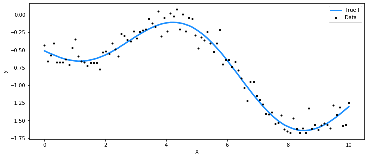
## Plot the data and the unobserved latent function
fig = plt.figure(figsize=(12,5)); ax = fig.gca()
ax.plot(X, f_true, "dodgerblue", lw=3, label="True f")
ax.plot(X, y, 'ok', ms=3, label="Data")
ax.set_xlabel("X"); ax.set_ylabel("y"); plt.legend();

png

@pm.model
def latent_gp_model(X, y, X_new):
    """A latent GP model with unknown length_scale and student-t noise

    Parameters
    ----------
    X: np.ndarray, tensor
        The prior data
    y: np.ndarray, tensor
        The function corresponding to the prior data
    X_new: np.ndarray, tensor
        The new data points to evaluate the conditional

    Returns
    -------
    y_: tensor
        Random sample from inferred function and its noise.
    """
    # We define length_scale of RBF kernel as a random variable
    l = yield pm.HalfCauchy("l", scale=5.)
    # We can now define a GP with mean as zeros and covariance function
    # as RBF kernel with ``length_scale=l`` and ``amplitude=1``
    cov_fn = pm.gp.cov.ExpQuad(length_scale=l, amplitude=1., feature_ndims=1)
    latent_gp = pm.gp.LatentGP(cov_fn=cov_fn)
    # f is the prior and f_pred is the conditional which we discussed in theory section
    f = yield latent_gp.prior("f", X=X)
    f_pred = yield latent_gp.conditional("f_pred", X_new, given={'X': X, 'f': f})
    # finally, we model the noise and our outputs.
    ν = yield pm.Gamma("ν", concentration=1., rate=0.1)
    y_ = yield pm.StudentT("y", loc=f, scale=0.1, df=ν, observed=y)
    return y_


gp = latent_gp_model(X, y, X_new)
trace = pm.sample(gp, num_samples=1000, num_chains=1)
trace.posterior

<pre>&lt;xarray.Dataset&gt;
Dimensions:                       (chain: 1, draw: 1000, latent_gp_model/f_dim_0: 100, latent_gp_model/f_pred_dim_0: 200)
Coordinates:
  * chain                         (chain) int32 0
  * draw                          (draw) int32 0 1 2 3 4 ... 995 996 997 998 999
  * latent_gp_model/f_dim_0       (latent_gp_model/f_dim_0) int32 0 1 ... 98 99
  * latent_gp_model/f_pred_dim_0  (latent_gp_model/f_pred_dim_0) int32 0 ... 199
Data variables:
    latent_gp_model/f             (chain, draw, latent_gp_model/f_dim_0) float32 -0.50917363 ... -1.3819383
    latent_gp_model/f_pred        (chain, draw, latent_gp_model/f_pred_dim_0) float32 -0.48531333 ... 0.4299915
    latent_gp_model/__log_l       (chain, draw) float32 1.1554403 ... 1.0889233
    latent_gp_model/__log_ν       (chain, draw) float32 2.1579044 ... 2.1388285
    latent_gp_model/l             (chain, draw) float32 3.1754212 ... 2.9710734
    latent_gp_model/ν             (chain, draw) float32 8.652986 ... 8.489487
Attributes:
    created_at:  2020-03-15T07:50:30.568276</pre>

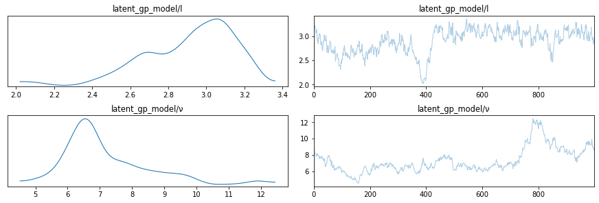
lines = [
    ("l", {}, l_true),
    ("ν", {}, ν_true),
]
az.plot_trace(trace, lines=lines, var_names=["latent_gp_model/l", "latent_gp_model/ν"])

array([[<matplotlib.axes._subplots.AxesSubplot object at 0x000001BCCCF73780>,
        <matplotlib.axes._subplots.AxesSubplot object at 0x000001BCC6764438>],
        [<matplotlib.axes._subplots.AxesSubplot object at 0x000001BCC567FEB8>,
        <matplotlib.axes._subplots.AxesSubplot object at 0x000001BCC9BB0128>]],
        dtype=object)

png

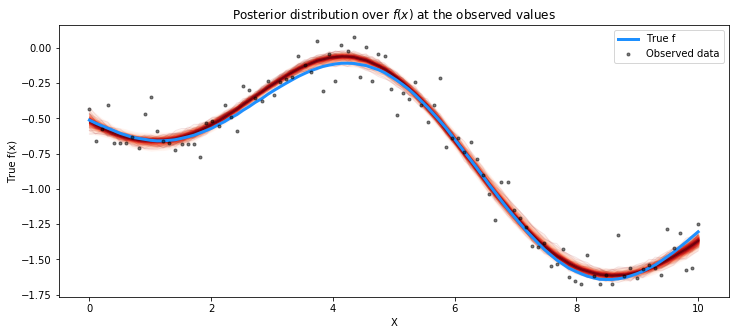
from pymc4.gp.util import plot_gp_dist
# plot the results
fig = plt.figure(figsize=(12,5)); ax = fig.gca()

# plot the samples from the gp posterior with samples and shading
plot_gp_dist(ax, np.array(trace.posterior["latent_gp_model/f"])[0], X)

# plot the data and the true latent function
plt.plot(X, f_true, "dodgerblue", lw=3, label="True f")
plt.plot(X, y, 'ok', ms=3, alpha=0.5, label="Observed data")

# axis labels and title
plt.xlabel("X"); plt.ylabel("True f(x)")
plt.title("Posterior distribution over $f(x)$ at the observed values"); plt.legend();

png

pred_samples = pm.sample_posterior_predictive(gp, trace=trace, var_names=["latent_gp_model/f_pred"])
pred_samples.posterior_predictive

<pre>&lt;xarray.Dataset&gt;
Dimensions:                       (chain: 1, draw: 1000, latent_gp_model/f_pred_dim_0: 200)
Coordinates:
  * chain                         (chain) int32 0
  * draw                          (draw) int32 0 1 2 3 4 ... 995 996 997 998 999
  * latent_gp_model/f_pred_dim_0  (latent_gp_model/f_pred_dim_0) int32 0 ... 199
Data variables:
    latent_gp_model/f_pred        (chain, draw, latent_gp_model/f_pred_dim_0) float32 -0.48531333 ... 0.4299915
Attributes:
    created_at:  2020-03-15T07:51:00.033659</pre>

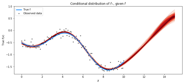
fig = plt.figure(figsize=(12,5)); ax = fig.gca()
plot_gp_dist(ax, pred_samples.posterior_predictive["latent_gp_model/f_pred"][0], X_new)
plt.plot(X, f_true, "dodgerblue", lw=3, label="True f")
plt.plot(X, y, 'ok', ms=3, alpha=0.5, label="Observed data")
plt.xlabel("$X$"); plt.ylabel("True $f(x)$")
plt.title("Conditional distribution of $f_*$, given $f$"); plt.legend();

png