Kernels for GP Modelling in PyMC4.
In this tutorial, we will explore the covariance functions aka kernels present in pm.gp module and study their properties. This will help choose the appropriate kernel to model your data properly. We will also see the semantics of additive and multiplicative kernels.
import arviz as az
import matplotlib.pyplot as plt
import matplotlib.cm as cmap
import numpy as np

import pymc4 as pm
from pymc4.gp.cov import *
from pymc4.gp.util import stabilize

import tensorflow as tf

from utils import plot_samples, plot_cov_matrix
%config InlineBackend.figure_format = 'retina'
RANDOM_SEED = 4200
tf.random.set_seed(RANDOM_SEED)
az.style.use('arviz-darkgrid')
Basic API Walkthrough
Let’s start with a basic kernel called the constant kernel. Using this kernel, I will walk you through the basic API for working with any kernel function in GP.
The constant kernel just evaluates to a constant value in each entry of the covariance matrix irrespective of the input. It is very useful as a lightweight kernel when speed and performance is a primary goal. It doesn’t evaluate a complex function and so its gradients are faster and easier to compute.
The mathematical formula of the constant kernel is pretty straight forward:
The signature of the constant kernel implemented in pymc4 is:
K = Constant(coef, feature_ndims=1, active_dims=None, scale_diag=None)
The first argument coef to the constructor is the constant value c which represents the covariance between any two points. Thus, the covariance matrix just evaluates to this constant value.
The argument feature_ndims is the number of feature dimensions of the input between which you want to evaluate the covariance. We will see the effect of this argument later.
The third argument active_dims is the feature or the number of features of each of the feature_ndims number of feature dimensions that will be considered during the computation. We will explore this in detail later.
The last argument scale_diag is used to perform Automatic Relevance Determination (ARD) and is a scaling factor of the length_scale parameter of stationary covariance kernels.
One important boolean keyword argument is ARD that tells pymc4 whether or not to perform ARD while modeling GPs. Its default value is True. A little overhead is incurred when ARD is enabled.
These four arguments feature_ndims, active_dims, scale_diag, and ARD are common in all the kernels implemented in pymc4 and optional.
Other keywords arguments that can be passed are:
- validate_args: A boolean indicating whether or not to validate arguments. Incurs a little overhead when set to True. Its default value is False.
- name: You can optionally give a name to the kernels. All the operations will be preformed under that name.
coef = 1.0

k = Constant(coef=coef, ARD=False)
We can call the kernel object k to evaluate the covariance matrix between two arrays or tensors of points. It outputs a covariance matrix which is a tf.Tensor object.
It accepts any inputs with the shape of the form (batch_shapes_1, m, features_1) and (batch_shapes_2, n, features_2). batch_shapes_1 is the batch shape of the first tensor and batch_shapes_2 is the batch shape of the second tensor. Multiple batches can be stacked together. Batch shapes must be equal or broadcastable according to the numpy’s rules for broadcasting. features_1 and features_2 are the feature dimensions and their length must be equal to feature_ndims. The feature dimensions don’t need to be broadcastable. When the kernel object k is called on such inputs, it outputs a tensor of shape (broadcasted_batch_shapes, m, n) where broadcasted_batch_shapes is the broadcasted batch shape.
As an outer product is taken along all the entries of each feature_ndims dimensions, the output doesn’t contain these dimensions. Hence, having two feature dimensions of shape (3, 3) yields the same result as having a single feature dimension with all the 9 nine entries.
For example, take two inputs with the following shape:
x1 has shape `(5, 4, 1, 40, 2, 2)`
x2 has shape `(5, 1, 3, 80, 2, 2)`
              |______| |__| |___|
                 |      |     |
       batch_shapes     |   feature_ndims
                      points
Such input will produce an output of shape:
k(x1, x2) has shape `(5, 4, 3, 40, 80)`
                     |______| |__||__|
                        |      |   |
  broadcasted_batch_shapes     |   points in x2
                      points in x1
Let’s see some more examples
Example 1 : Only one batch and one feature dimension.
x1 = np.array([[1.0, 2.0], [3.0, 4.0]])
x2 = np.array([[5.0, 6.0], [7.0, 8.0]])

k(x1, x2)
<tf.Tensor: shape=(2, 2), dtype=float32, numpy=
array([[1., 1.],
        [1., 1.]], dtype=float32)>
Example 2 : Multiple batch dimensions and one feature dimension
Let’s batch two tensors of shape (2, 2) and call the kernel with that
batched_x1 = np.array([[[1.0, 2.0], [3.0, 4.0]], [[5.0, 6.0], [7.0, 8.0]]])
batched_x2 = np.array([[[9.0, 10.0], [11.0, 12.0]], [[13.0, 14.0], [15.0, 16.0]]])

print(batched_x1.shape)
print(batched_x2.shape)
print(k(batched_x1, batched_x2))
(2, 2, 2)
(2, 2, 2)
tf.Tensor(
[[[1. 1.]
    [1. 1.]]

    [[1. 1.]
    [1. 1.]]], shape=(2, 2, 2), dtype=float32)
Example 3 : Multiple batches and feature dimensions
The below example has 2 batch dimensions and 2 feature dimensions. So the output will have a shape with the first two dimensions being the batch dimensions and the other two dimensions being the number of examples in each tensor. The feature_ndims are absorbed during the computation.
# Notice that the batch shape is broadcatable but the
# feature dimensions need not be broadcastable.
batched_x1 = np.random.randn(5, 4, 1, 40, 3, 3)
batched_x2 = np.random.randn(5, 1, 3, 80, 2, 2)

k = Constant(coef=coef, feature_ndims=2, ARD=False)

print(batched_x1.shape)
print(batched_x2.shape)
print(k(batched_x1, batched_x2).shape)
(5, 4, 1, 40, 3, 3)
(5, 1, 3, 80, 2, 2)
(5, 4, 3, 40, 80)
Note: It is not recommended to work with multiple feature dimensions as it incurs a substantial overhead.
%timeit k(batched_x1, batched_x2)
2 ms ± 56.8 µs per loop (mean ± std. dev. of 7 runs, 100 loops each)
# Let's see how it performs with a single feature dimension.

batched_x1 = batched_x1.reshape(5, 4, 1, 40, 9)
batched_x2 = batched_x2.reshape(5, 1, 3, 80, 4)

k = Constant(coef=coef, feature_ndims=1, ARD=False)

%timeit k(batched_x1, batched_x2)
2.01 ms ± 54.8 µs per loop (mean ± std. dev. of 7 runs, 100 loops each)
Example 4: Active Dimensions
Active dimensions are (as the name suggests) active dimensions of each feature dimension which will be used during the computation of the covariance matrix. This sounds too complicated but easy to understand with an example. Let’s say we have two feature dimensions of size (10, ) and (20, ). This means that our input is going to be of shape (..., m, 10, 20) and (..., n, 10, 20).
Active dimensions allows you to choose only those dimensions that you want the kernel to use to calculate the covariance matrix. For example, active_dims=[5, 10] means the first 5 entries of the first feature dimension and the first 10 entries of the second feature dimension will be used during the computation.
active_dims = [5, 10]

x1 = tf.random.normal((4, 10, 20))
x2 = tf.random.normal((5, 10, 20))

k = ExpQuad(length_scale=10.0, feature_ndims=2, active_dims=active_dims, ARD=False)

k(x1, x2)
<tf.Tensor: shape=(4, 5), dtype=float32, numpy=
array([[0.671924  , 0.60107315, 0.6406969 , 0.5356703 , 0.61101484],
        [0.6593888 , 0.6020972 , 0.68694246, 0.6295366 , 0.5677304 ],
        [0.6531334 , 0.6526655 , 0.65813994, 0.55865365, 0.5552639 ],
        [0.6973517 , 0.5949804 , 0.689168  , 0.6187942 , 0.6739167 ]],
        dtype=float32)>
You can also pick the entries you want to be active for each feature dimension.
For example, active_dims=[[1, 4, 5], 10] means 2’nd, 5’th, and 6’th entries are active in the first feature dimension and the first 10 entries are active in the second feature dimension.
active_dims = [[1, 4, 5], 10]

x1 = tf.random.normal((4, 10, 20))
x2 = tf.random.normal((5, 10, 20))

k = ExpQuad(length_scale=10.0, feature_ndims=2, active_dims=active_dims, ARD=False)

k(x1, x2)
<tf.Tensor: shape=(4, 5), dtype=float32, numpy=
array([[0.7338076 , 0.7271027 , 0.63948095, 0.74313736, 0.6497098 ],
        [0.76253086, 0.7478951 , 0.71348906, 0.7848295 , 0.8584582 ],
        [0.7686134 , 0.7458844 , 0.6849413 , 0.828126  , 0.74713683],
        [0.75363666, 0.80211973, 0.64971805, 0.80924386, 0.74323034]],
        dtype=float32)>
Scale Diag
This is the scaling factor for the length_scale parameter present in the stationary kernels that come from Squared Exponential, Rational Quadratic, Matern, and Periodic families. It is ignored if ARD=False.
It is used to perform Automatic Relevance Determination (ARD) on stationary kernels. This parameter can be inferred during sampling or MAP estimation.
x1 = tf.constant([[1.0, 2.0], [3.0, 4.0]])
x2 = tf.constant([[1.0, 2.0], [3.0, 4.0]])

k = ExpQuad(length_scale=1.0, feature_ndims=1, ARD=False)

print(k(x1, x2))

k = ExpQuad(length_scale=1.0, feature_ndims=1, scale_diag=2.0, ARD=False)

print(k(x1, x2))
tf.Tensor(
[[1.         0.01831564]
    [0.01831564 1.        ]], shape=(2, 2), dtype=float32)
tf.Tensor(
[[1.         0.01831564]
    [0.01831564 1.        ]], shape=(2, 2), dtype=float32)
As you can see, the off-diagonal entries got scaled by 2 because scale_diag was 2.
Stationary Kernels in PyMC4!
PyMC4 implements 8 stationary kernels which are used extensively in Gaussian Process modeling. These kernels don’t change their parameter values at different points in space.
The stationary kernels implemented in PyMC4 are:
- Constant Kernel
- White Noise Kernel
- Exponential Quadratic Kernel
- Rational Quadratic Kernel
- Matern 1/2 Kernel
- Matern 3/2 Kernel
- Matern 5/3 Kernel
- Exponential Kernel
Constant Kernel
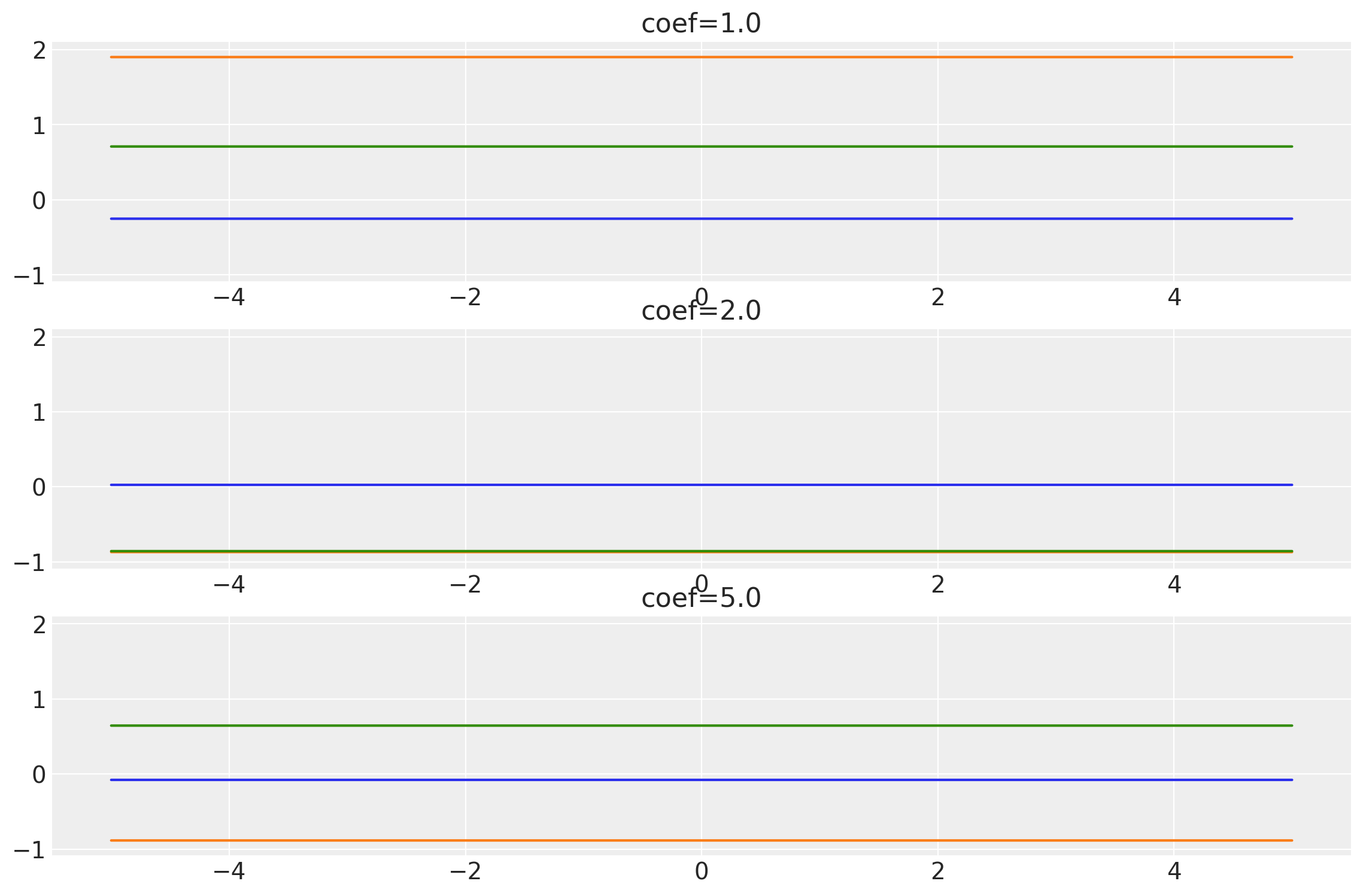
As we have seen above, the constant kernel is a lightweight constant function and gradients are easy to calculate. Now, let’s look at the function space and the covariance matrix.
# This is a batch of coefficients. You can batch several
# constant kernels together for fast vectorized computations.
coefs = tf.constant([1.0, 2.0, 5.0], dtype=tf.float64)

k = Constant(coef=coefs, ARD=False)
x = np.linspace(-5, 5, num=100)[:, np.newaxis]

# We stabilize the kernel to make it Positive Semi-Definite.
# It just adds a small shift to the diagonal entries and is
# necessary to sample from the MvNormal distribution.
covs = stabilize(k(x, x), shift=1e-13)
dists = pm.MvNormal("_", loc=0.0, covariance_matrix=covs)
samples = tf.transpose(dists.sample(3), perm=[1, 0, 2])
plot_samples(x, samples, labels=coefs, names="coef")
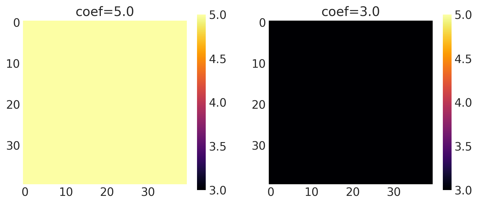
x1, x2 = np.meshgrid(np.linspace(-1, 1, 10), np.linspace(-1, 1, 4))
X2 = np.concatenate((x1.reshape(40, 1), x2.reshape(40, 1)), axis=1)

coef = [5.0, 3.0]
k = Constant(coef=coef, ARD=False)

plot_cov_matrix(k, X2, [coef], ["coef"])
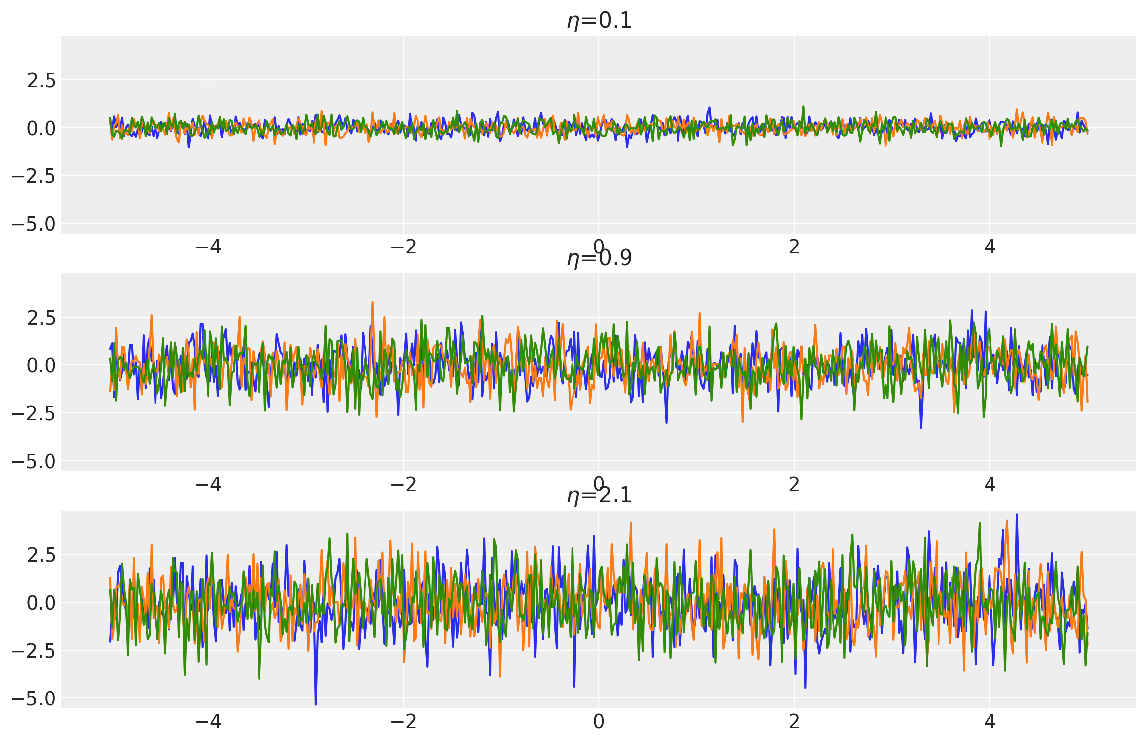
White Noise Kernel
This kernel adds some noise to the covariance functions and is mostly
used to stabilize other Positive Semi-Definite (PSD) kernels. This helps them become non-singular
and makes cholesky decomposition possible for sampling from the
MvNormalCholesky distribution. It is recommended to use this kernel in
combination with other covariance/kernel function when working with GP on
large data.
where \(\eta^2\) is ‘noise level’ or simply noise.
The signature of WhiteNoise kernel implemented in pymc4 is:
k = WhiteNoise(noise, feature_ndims=1., active_dims=None, scale_diag=None)
noises = tf.constant([0.1, 0.9, 2.1])

k = WhiteNoise(noise=noises, ARD=False)
x = np.linspace(-5, 5, num=500)[:, np.newaxis]

covs = stabilize(k(x, x), shift=1e-6)
dists = pm.MvNormal("_", loc=0.0, covariance_matrix=covs)
samples = tf.transpose(dists.sample(3), perm=[1, 0, 2])
plot_samples(x, samples, noises, "$\\eta$")
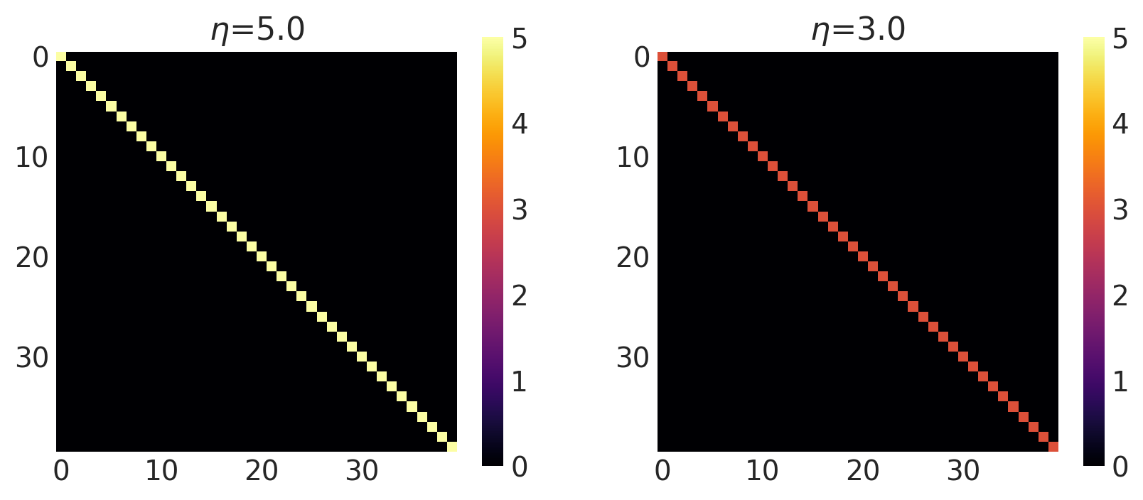
x1, x2 = np.meshgrid(np.linspace(-1, 1, 10), np.linspace(-1, 1, 4))
X2 = np.concatenate((x1.reshape(40, 1), x2.reshape(40, 1)), axis=1)

noise = [5.0, 3.0]
k = WhiteNoise(noise=noise, ARD=False)

plot_cov_matrix(k, X2, [noise], ["$\\eta$"])
Exponential Quadratic Kernel
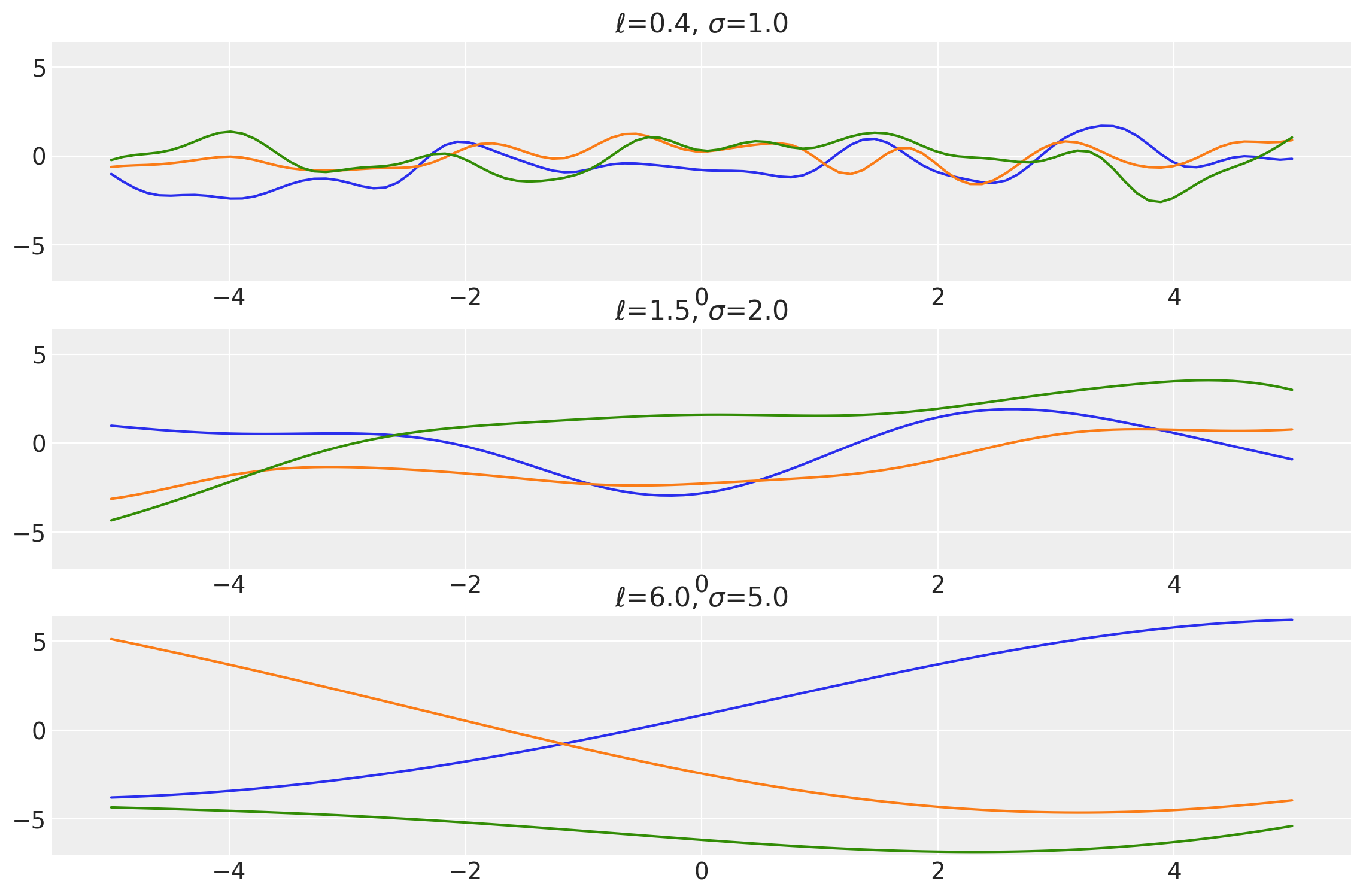
This is the most used kernel in GP Modelling because of its mathematical properties. It is infinitely differentiable and forces the covariance function to be smooth. It comes from Squared Exponential (SE) family of kernels which is also commonly called as the Radial Basis Kernel (RBF) Family.
It’s mathematical expression is:
where \(\sigma\) is called “amplitude” and \(\ell\) is called “length scale” of the kernel.
Amplitude controls how many units away the covariance is from the mean and length scale controls the ‘wiggles’ in the function prior. In general, you won’t be able to extrapolate more than ℓ units away from your data. If a float, an isotropic kernel is used. If an array and ARD=True, an anisotropic kernel is used where each dimension defines the length-scale of the respective feature dimension.
The signature of Exponential Quadratic kernel implemented in pymc4 is:
k = ExpQuad(length_scale=1., amplitude=1., feature_ndims=1, active_dims=None, scale_diag=None)
# We are using tf.float64 for better numerical accuracy.
length_scales = tf.constant([0.4, 1.5, 6.0], dtype=tf.float64)
amplitudes = tf.constant([1.0, 2.0, 5.0], dtype=tf.float64)

k = ExpQuad(length_scale=length_scales, amplitude=amplitudes, ARD=False)
x = np.linspace(-5, 5, num=100)[:, np.newaxis]

covs = stabilize(k(x, x), shift=1e-8)
dists = pm.MvNormal("_", loc=0.0, covariance_matrix=covs)
samples = tf.transpose(dists.sample(3), perm=[1, 0, 2])
plot_samples(x, samples, [length_scales, amplitudes], ["$\\ell$", "$\\sigma$"])
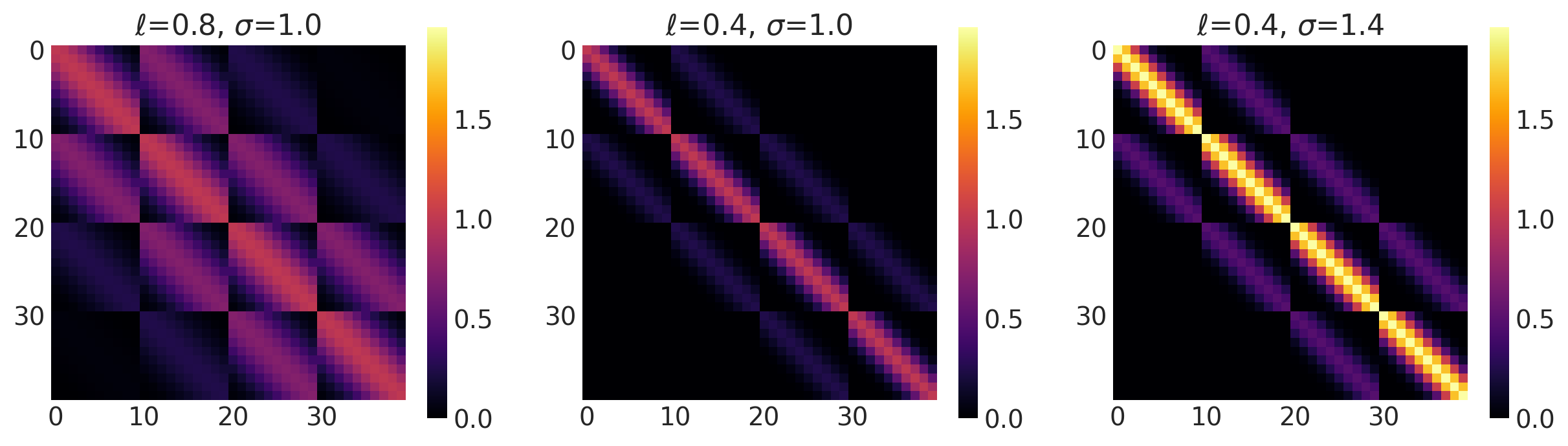
x1, x2 = np.meshgrid(np.linspace(-1, 1, 10), np.linspace(-1, 1, 4))
X2 = np.concatenate((x1.reshape(40, 1), x2.reshape(40, 1)), axis=1)

ls, amp = [0.8, 0.4, 0.4], [1.0, 1.0, 1.4]
k = ExpQuad(length_scale=ls, amplitude=amp, ARD=False)

plot_cov_matrix(k, X2, [ls, amp], ["$\\ell$", "$\\sigma$"])
Rational Quadratic Kernel
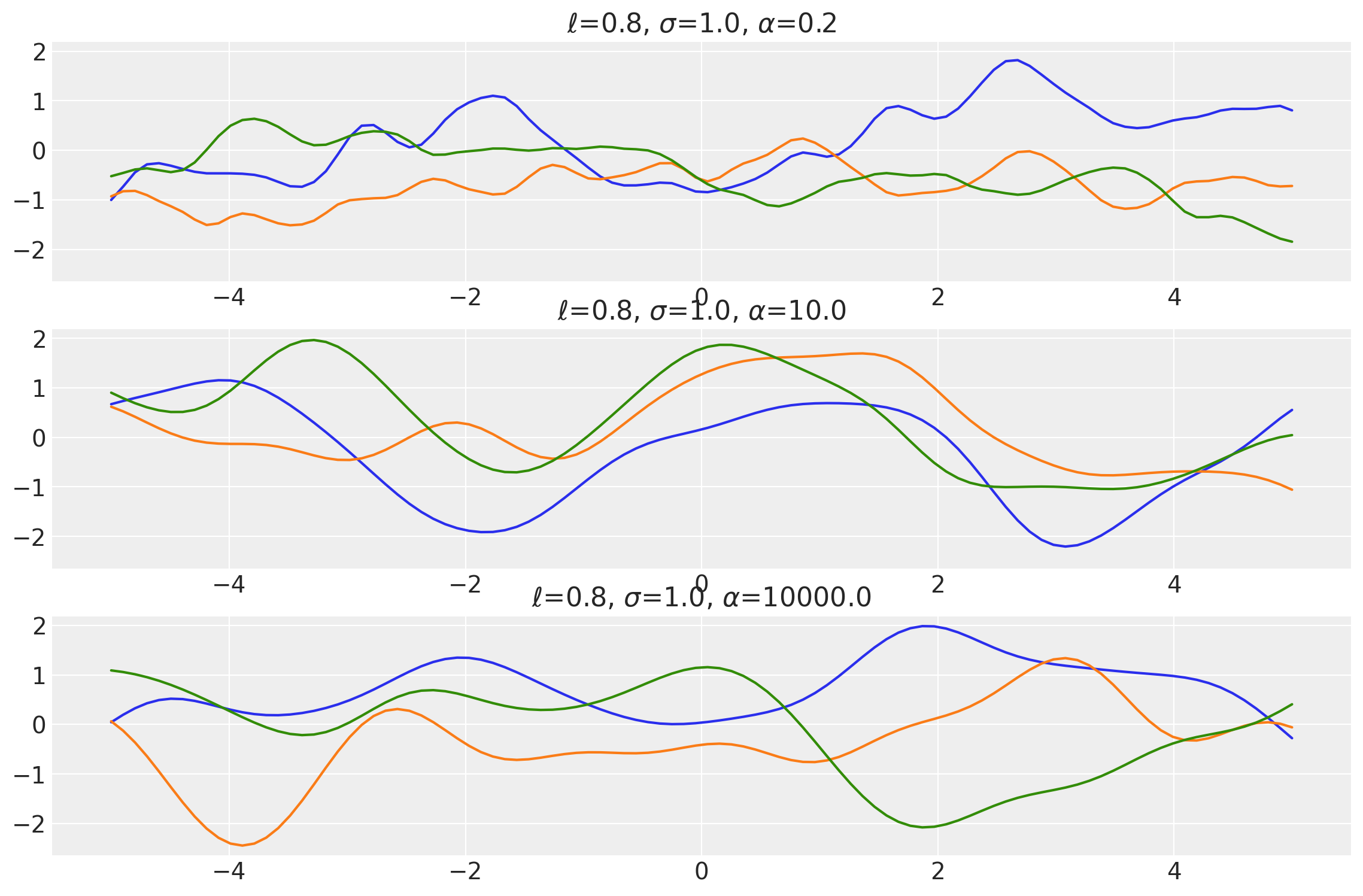
Rational Quadratic Kernel is a generalization over the Exponential Quadratic Kernel. It is equivalent to using a combination of Exponential Quadratic kernel with different length scales. One extra parameter \(\alpha\) controls the “mixture rate” of the kernel and is also known as “scale mixture rate”. As this parameter approaches infinity, the kernel becomes exactly equivalent to the Exponential Quadratic Kernel. The mathematical formula for the kernel is given by:
where \(\sigma\) is the amplitude, \(\ell\) is the length scale, and \(\alpha\) is the scale mixture rate.
The signature of the kernel implemented in pymc4 is:
k = RatQuad(length_scale, amplitude=1., scale_mixture_rate=1., feature_ndims=1, active_dims=None, scale_diag=None)
length_scales = tf.constant([0.8, 0.8, 0.8], dtype=tf.float64)
amplitudes = tf.constant([1.0, 1.0, 1.0], dtype=tf.float64)
scale_mixture_rates = tf.constant([0.2, 10.0, 10000.0], dtype=tf.float64)

k = RatQuad(
    length_scale=length_scales,
    amplitude=amplitudes,
    scale_mixture_rate=scale_mixture_rates,
    ARD=False,
)
x = np.linspace(-5, 5, num=100)[:, np.newaxis]

covs = stabilize(k(x, x), shift=1e-8)
dists = pm.MvNormal("_", loc=0.0, covariance_matrix=covs)
samples = tf.transpose(dists.sample(3), perm=[1, 0, 2])
plot_samples(
    x,
    samples,
    [length_scales, amplitudes, scale_mixture_rates],
    ["$\\ell$", "$\\sigma$", "$\\alpha$"],
)
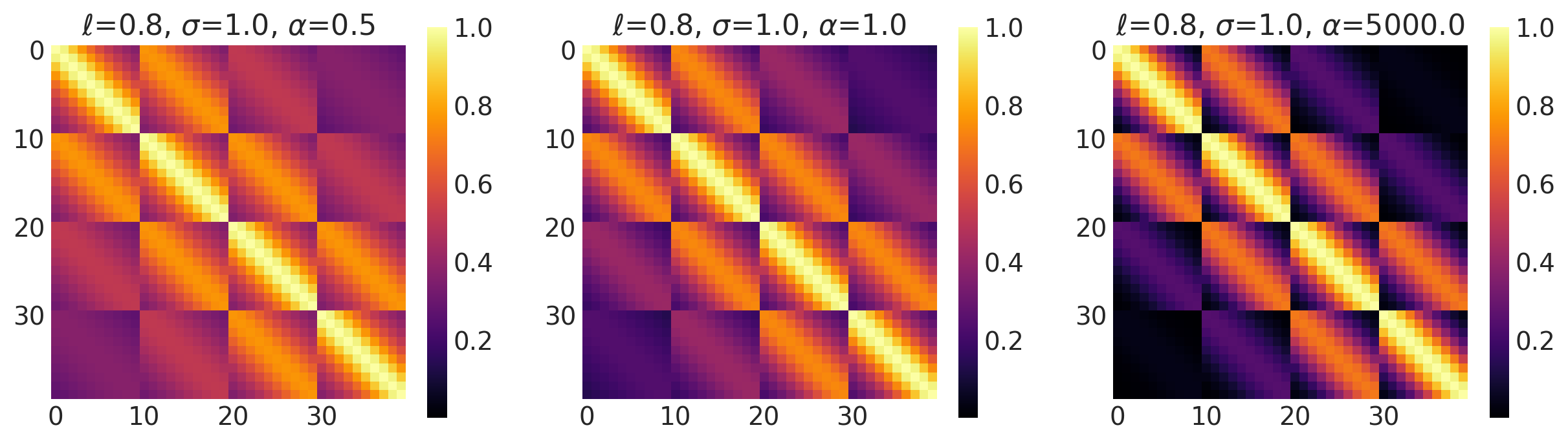
x1, x2 = np.meshgrid(np.linspace(-1, 1, 10), np.linspace(-1, 1, 4))
X2 = np.concatenate((x1.reshape(40, 1), x2.reshape(40, 1)), axis=1)

ls, amp, alpha = [0.8, 0.8, 0.8], [1.0, 1.0, 1.0], [0.5, 1.0, 5000.0]
k = RatQuad(length_scale=ls, amplitude=amp, scale_mixture_rate=alpha, ARD=False)

plot_cov_matrix(k, X2, [ls, amp, alpha], ["$\\ell$", "$\\sigma$", "$\\alpha$"])
Matern Family of Kernels
Matern family of kernels is a generalization over the RBF family of kernels. The \(\nu\) parameter controls the smoothness of the kernel function. Higher values of \(\nu\) result in smoother functions. The most common values of \(\nu\) are 0.5, 1.5 and 2.5 as the modified Bessel’s function is analytical there. The full mathematical formula of matern kernels is given by:
where \(d(.)\) is the Euclidean distance, \(K_\nu(.)\) is a modified Bessel function and \(\Gamma(.)\) is the gamma function.
For other values of \(\nu\), the computational cost to evaluate the kernel is extremely high and so isn’t implemented in pymc4.
Let’s see the kernels we get for some special values of \(\nu\)
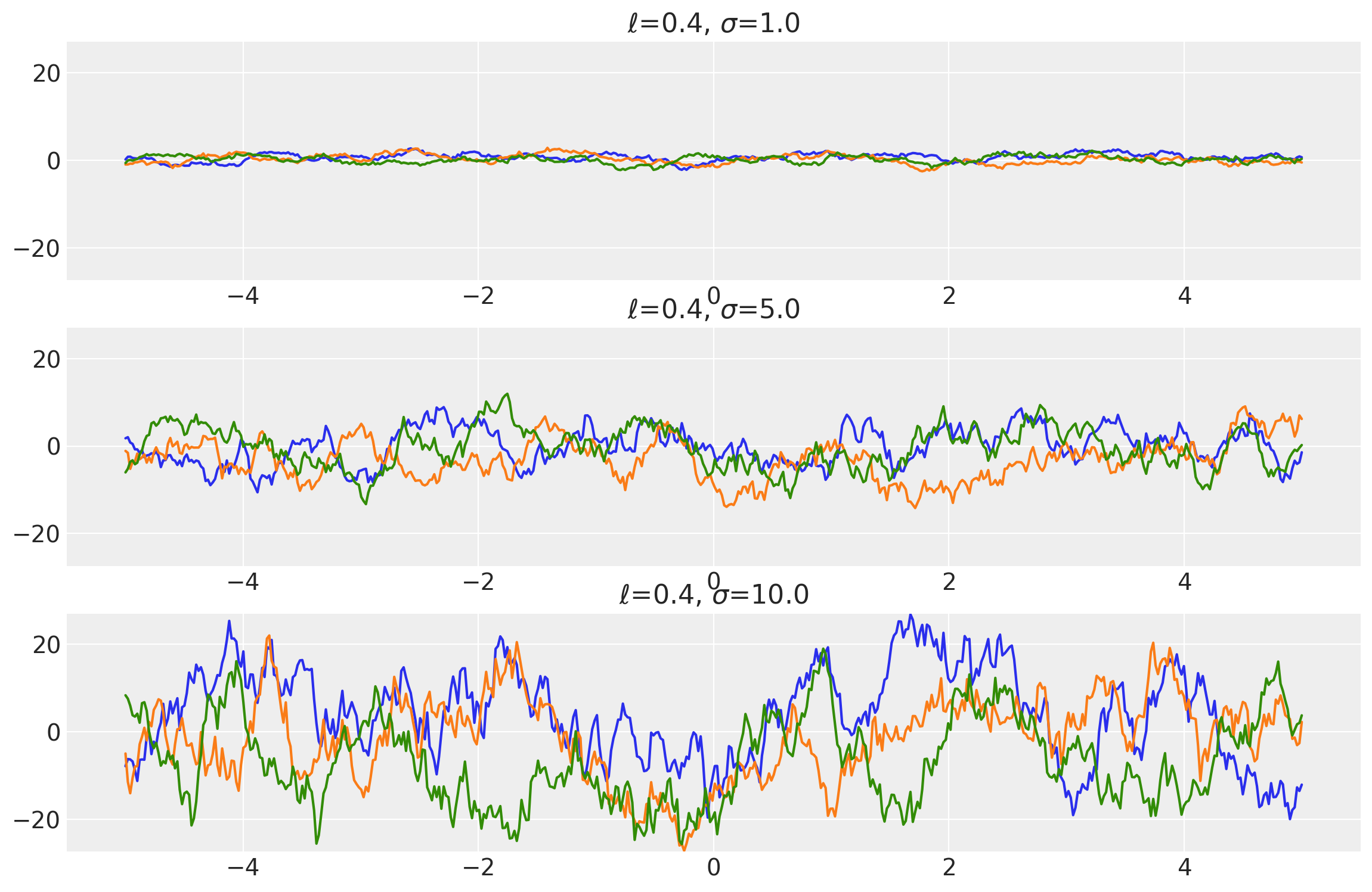
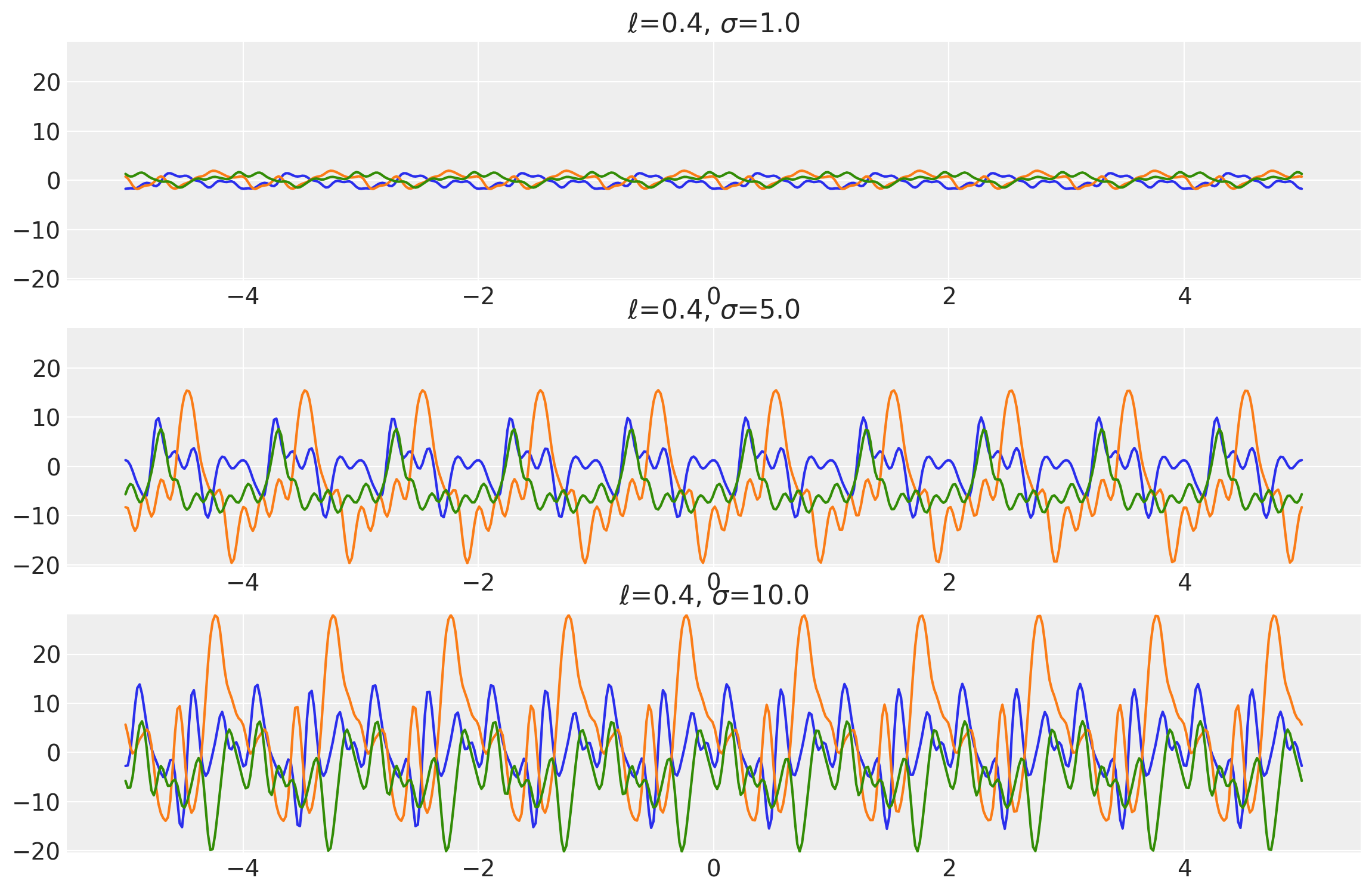
Matern 1/2 Kernel
This kernel has the value of \(\nu = 0.5\). It is used to model Ornstein-Uhlenbeck processes.
It is given by:
Its signature in pymc4 is:
k = Matern12(length_scale, amplitude=1., feature_ndims=1, active_dims=None, scale_diag=None)
Example 1
length_scales = tf.constant([0.4, 0.4, 0.4], dtype=tf.float64)
amplitudes = tf.constant([1.0, 5.0, 10.0], dtype=tf.float64)

k = Matern12(length_scale=length_scales, amplitude=amplitudes, ARD=False)
x = np.linspace(-5, 5, num=500)[:, np.newaxis]

covs = stabilize(k(x, x), shift=1e-8)
dists = pm.MvNormal("_", loc=0.0, covariance_matrix=covs)
samples = tf.transpose(dists.sample(3), perm=[1, 0, 2])
plot_samples(x, samples, [length_scales, amplitudes], ["$\ell$", "$\\sigma$"])
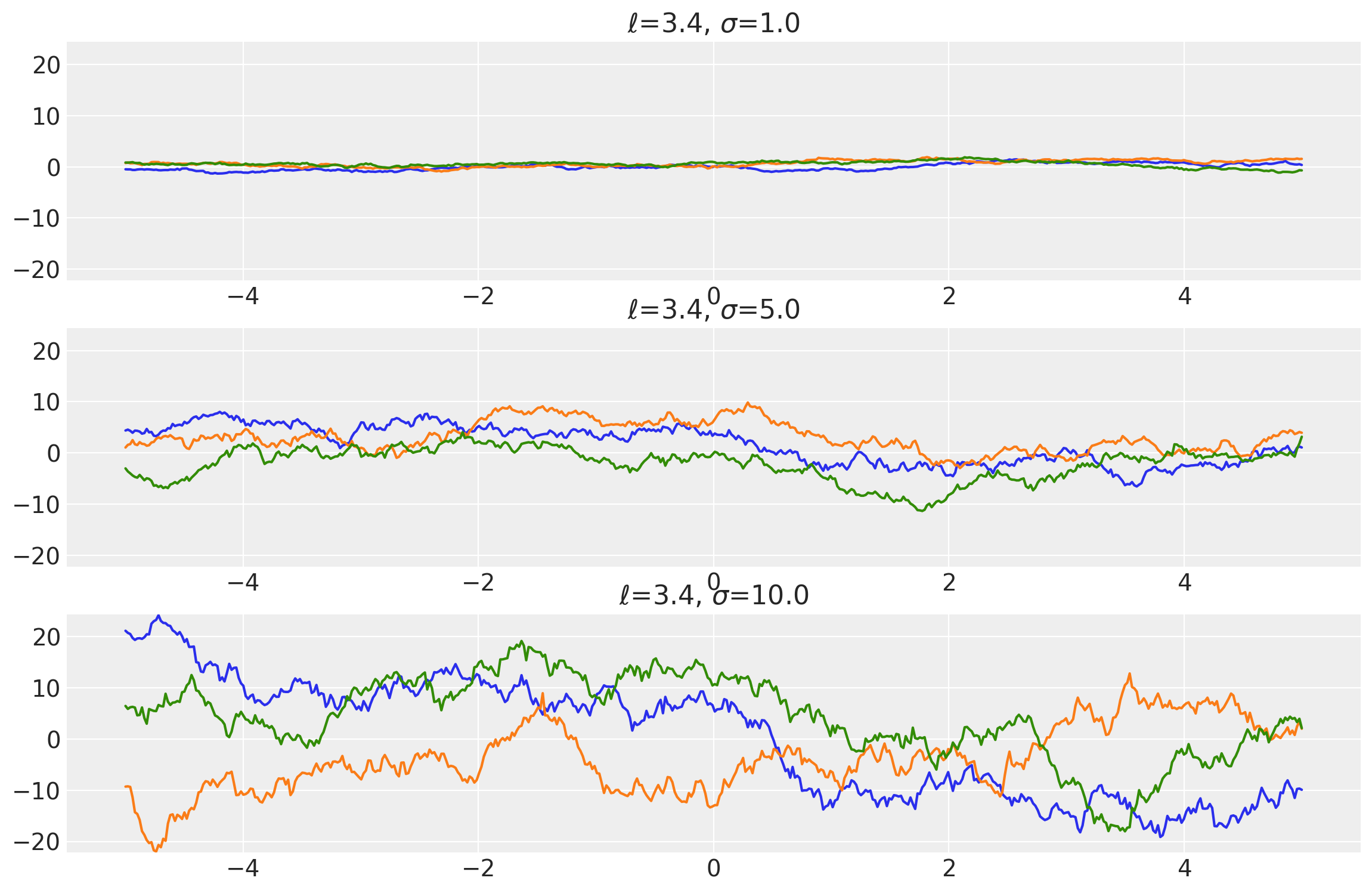
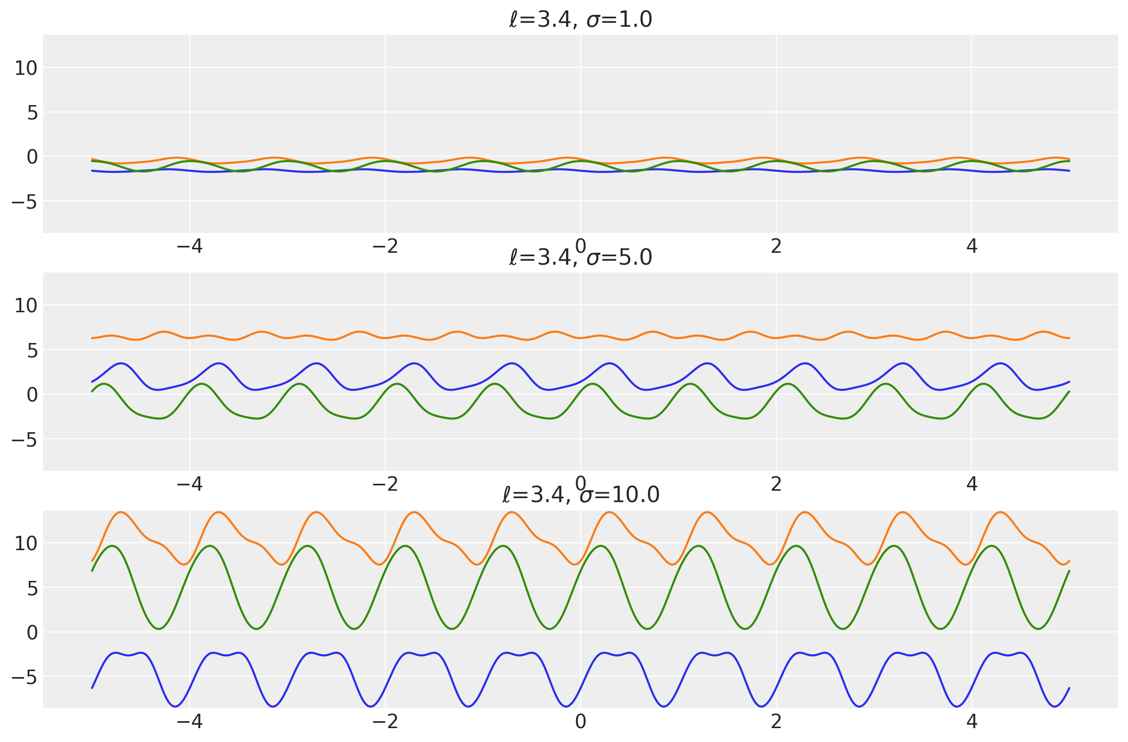
Example 2
length_scales = tf.constant([3.4, 3.4, 3.4], dtype=tf.float64)
amplitudes = tf.constant([1.0, 5.0, 10.0], dtype=tf.float64)

k = Matern12(length_scale=length_scales, amplitude=amplitudes, ARD=False)
x = np.linspace(-5, 5, num=500)[:, np.newaxis]

covs = stabilize(k(x, x), shift=1e-8)
dists = pm.MvNormal("_", loc=0.0, covariance_matrix=covs)
samples = tf.transpose(dists.sample(3), perm=[1, 0, 2])
plot_samples(x, samples, [length_scales, amplitudes], ["$\ell$", "$\\sigma$"])
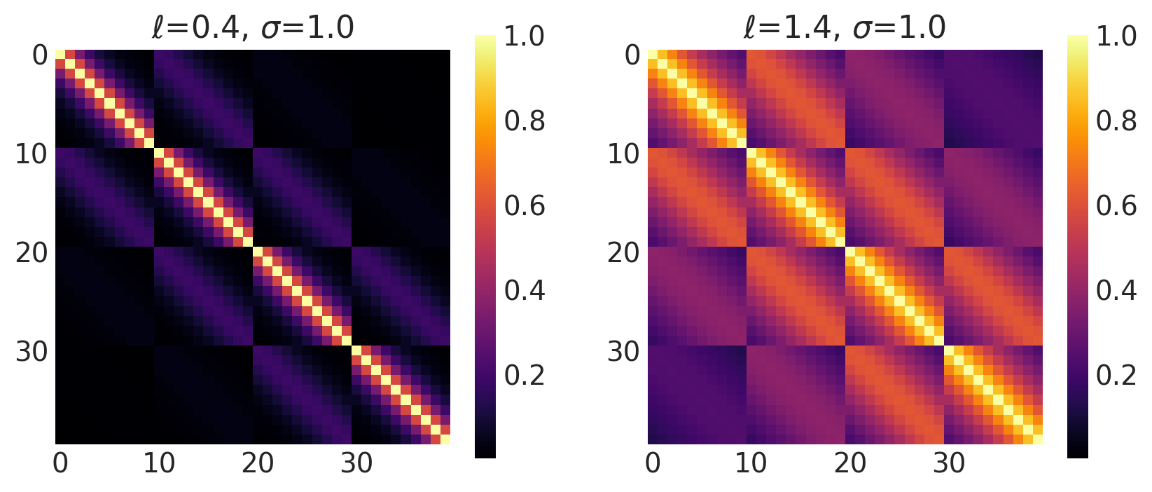
x1, x2 = np.meshgrid(np.linspace(-1, 1, 10), np.linspace(-1, 1, 4))
X2 = np.concatenate((x1.reshape(40, 1), x2.reshape(40, 1)), axis=1)

ls, amp = [0.4, 1.4], [1.0, 1.0]
k = Matern12(length_scale=ls, amplitude=amp, ARD=False)

plot_cov_matrix(k, X2, [ls, amp], ["$\\ell$", "$\\sigma$"])
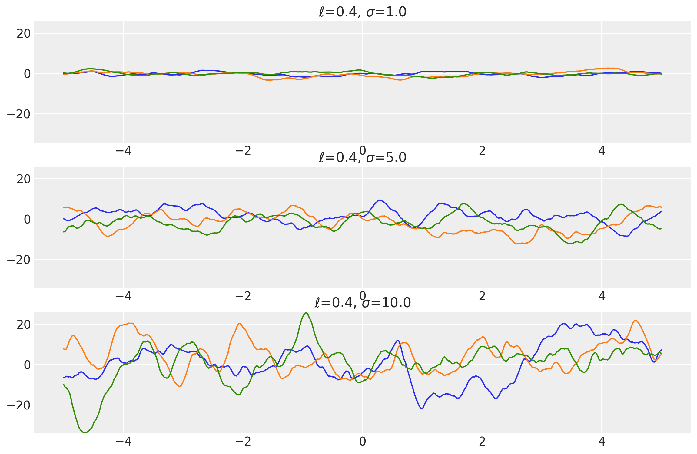
Matern 3/2 Kernel
This kernel has the value of \(\nu = 1.5\).
It is given by:
Its signature in pymc4 is:
k = Matern32(length_scale, amplitude=1., feature_ndims=1, active_dims=None, scale_diag=None)
Example 1
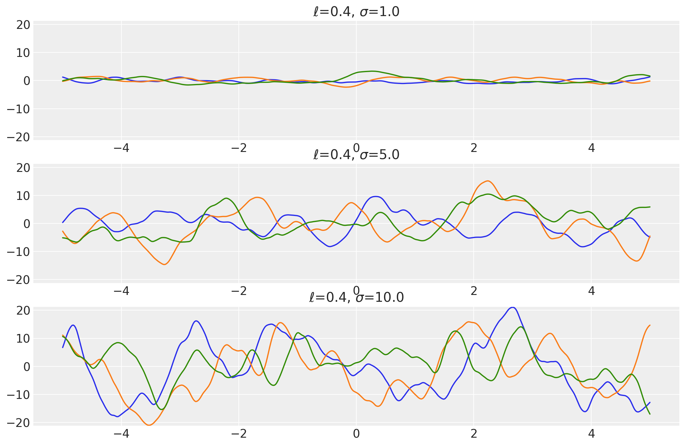
length_scales = tf.constant([0.4, 0.4, 0.4], dtype=tf.float64)
amplitudes = tf.constant([1.0, 5.0, 10.0], dtype=tf.float64)

k = Matern32(length_scale=length_scales, amplitude=amplitudes, ARD=False)
x = np.linspace(-5, 5, num=500)[:, np.newaxis]

covs = stabilize(k(x, x), shift=1e-8)
dists = pm.MvNormal("_", loc=0.0, covariance_matrix=covs)
samples = tf.transpose(dists.sample(3), perm=[1, 0, 2])
plot_samples(x, samples, [length_scales, amplitudes], ["$\\ell$", "$\\sigma$"])
Example 2
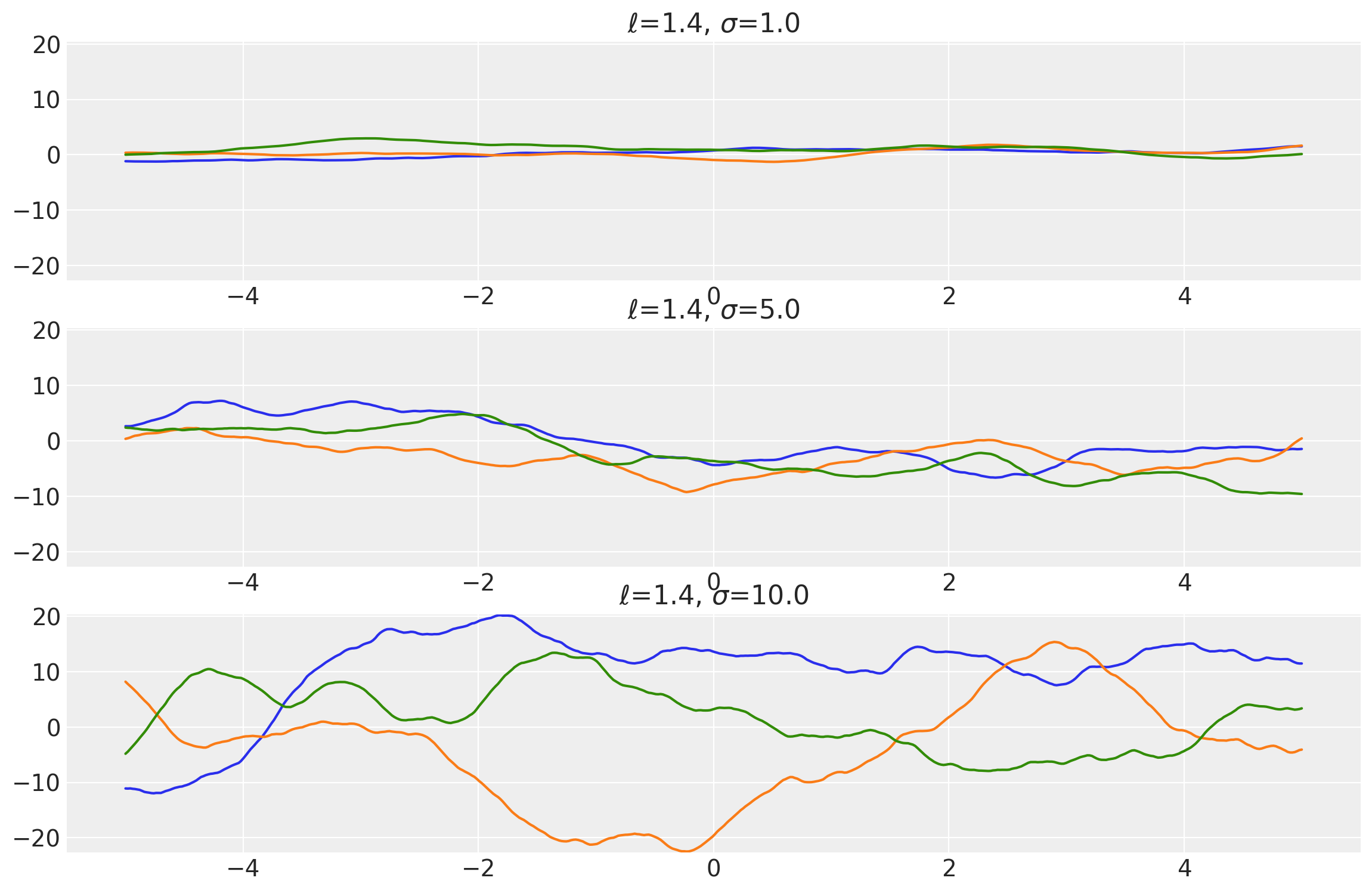
length_scales = tf.constant([1.4, 1.4, 1.4], dtype=tf.float64)
amplitudes = tf.constant([1.0, 5.0, 10.0], dtype=tf.float64)

k = Matern32(length_scale=length_scales, amplitude=amplitudes, ARD=False)
x = np.linspace(-5, 5, num=500)[:, np.newaxis]

covs = stabilize(k(x, x), shift=1e-8)
dists = pm.MvNormal("_", loc=0.0, covariance_matrix=covs)
samples = tf.transpose(dists.sample(3), [1, 0, 2])
plot_samples(x, samples, [length_scales, amplitudes], ["$\\ell$", "$\\sigma$"])
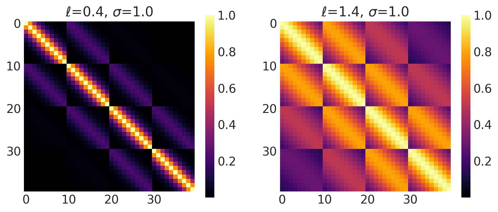
x1, x2 = np.meshgrid(np.linspace(-1, 1, 10), np.linspace(-1, 1, 4))
X2 = np.concatenate((x1.reshape(40, 1), x2.reshape(40, 1)), axis=1)

ls, amp = [0.4, 1.4], [1.0, 1.0]
k = Matern32(length_scale=ls, amplitude=amp, ARD=False)

plot_cov_matrix(k, X2, [ls, amp], ["$\\ell$", "$\\sigma$"])
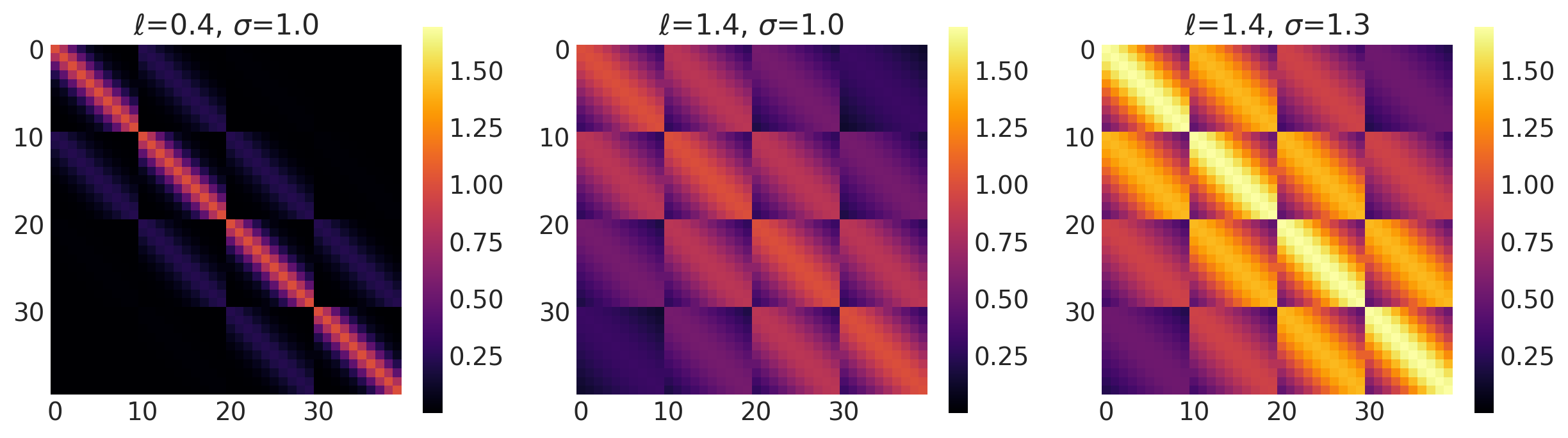
Matern 5/2 Kernel
This kernel has the value of \(\nu = 2.5\) It can be analytically shown as:
Its signature in PyMC4 is:
k = Matern52(length_scale, amplitude=1., feature_ndims=1, active_dims=None, scale_diag=None)
Example 1
length_scales = tf.constant([0.4, 0.4, 0.4], dtype=tf.float64)
amplitudes = tf.constant([1.0, 5.0, 10.0], dtype=tf.float64)

k = Matern52(length_scale=length_scales, amplitude=amplitudes, ARD=False)
x = np.linspace(-5, 5, num=500)[:, np.newaxis]

covs = stabilize(k(x, x), shift=1e-8)
dists = pm.MvNormal("_", loc=0.0, covariance_matrix=covs)
samples = tf.transpose(dists.sample(3), perm=[1, 0, 2])
plot_samples(x, samples, [length_scales, amplitudes], ["$\\ell$", "$\\sigma$"])
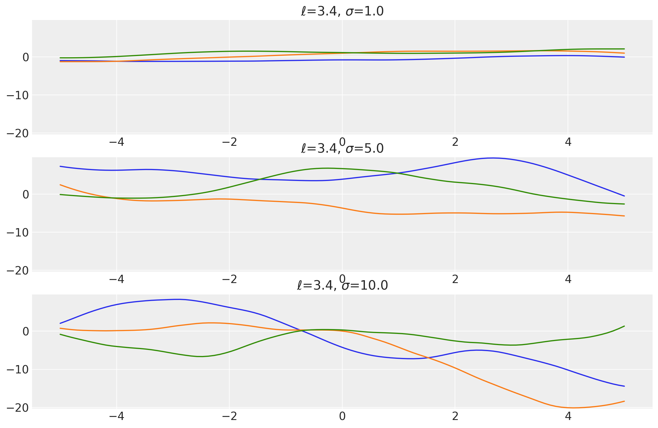
Example 2
length_scales = tf.constant([3.4, 3.4, 3.4], dtype=tf.float64)
amplitudes = tf.constant([1.0, 5.0, 10.0], dtype=tf.float64)

k = Matern52(length_scale=length_scales, amplitude=amplitudes, ARD=False)
x = np.linspace(-5, 5, num=100)[:, np.newaxis]

covs = stabilize(k(x, x), shift=1e-8)
dists = pm.MvNormal("_", loc=0.0, covariance_matrix=covs)
samples = tf.transpose(dists.sample(3), perm=[1, 0, 2])
plot_samples(x, samples, [length_scales, amplitudes], ["$\\ell$", "$\\sigma$"])
x1, x2 = np.meshgrid(np.linspace(-1, 1, 10), np.linspace(-1, 1, 4))
X2 = np.concatenate((x1.reshape(40, 1), x2.reshape(40, 1)), axis=1)

ls, amp = [0.4, 1.4, 1.4], [1.0, 1.0, 1.3]
k = Matern52(length_scale=ls, amplitude=amp, ARD=False)

plot_cov_matrix(k, X2, [ls, amp], ["$\\ell$", "$\\sigma$"])
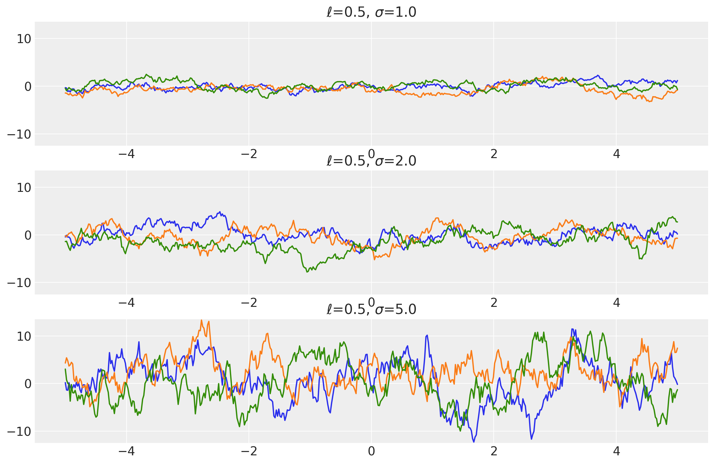
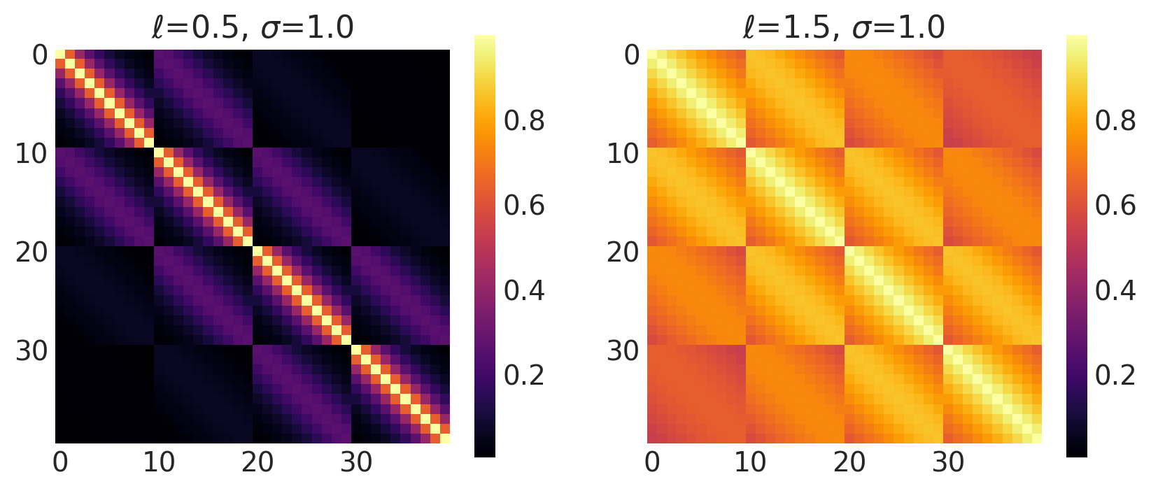
Exponential Kernel
It is also known as Laplacian kernel.
It’s mathematical formula can be given as:
The signature of this kernel is:
k = Exponential(length_scale, amplitude=1., feature_ndims=1, active_dims=None, scale_diag=None)
Example 1
length_scales = tf.constant([0.5, 0.5, 0.5], dtype=tf.float64)
amplitudes = tf.constant([1.0, 2.0, 5.0], dtype=tf.float64)

k = Exponential(length_scale=length_scales, amplitude=amplitudes, ARD=False)
x = np.linspace(-5, 5, num=500)[:, np.newaxis]

covs = stabilize(k(x, x), shift=1e-8)
dists = pm.MvNormal("_", loc=0.0, covariance_matrix=covs)
samples = tf.transpose(dists.sample(3), perm=[1, 0, 2])
plot_samples(x, samples, [length_scales, amplitudes], ["$\\ell$", "$\\sigma$"])
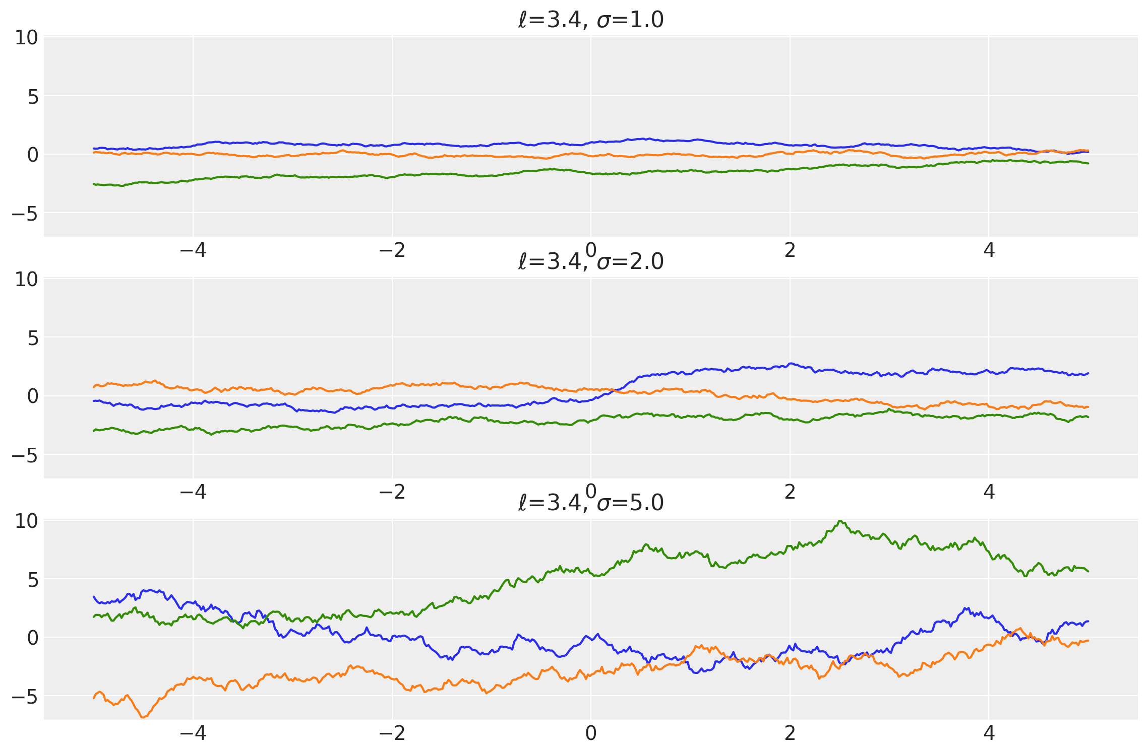
Example 2
length_scales = tf.constant([3.4, 3.4, 3.4], dtype=tf.float64)
amplitudes = tf.constant([1.0, 2.0, 5.0], dtype=tf.float64)

k = Exponential(length_scale=length_scales, amplitude=amplitudes, ARD=False)
x = np.linspace(-5, 5, num=500)[:, np.newaxis]

covs = stabilize(k(x, x), shift=1e-8)
dists = pm.MvNormal("_", loc=0.0, covariance_matrix=covs)
samples = tf.transpose(dists.sample(3), perm=[1, 0, 2])
plot_samples(x, samples, [length_scales, amplitudes], ["$\ell$", "$\\sigma$"])
x1, x2 = np.meshgrid(np.linspace(-1, 1, 10), np.linspace(-1, 1, 4))
X2 = np.concatenate((x1.reshape(40, 1), x2.reshape(40, 1)), axis=1)

ls, amp = [0.5, 1.5], [1.0, 1.0]
k = Exponential(length_scale=ls, amplitude=amp, ARD=False)

plot_cov_matrix(k, X2, [ls, amp], ["$\\ell$", "$\\sigma$"])
Periodic Kernels in PyMC4!
A total of 2 periodic kernels have been implemented in PyMC4.
Exponential Sine Squared Kernel
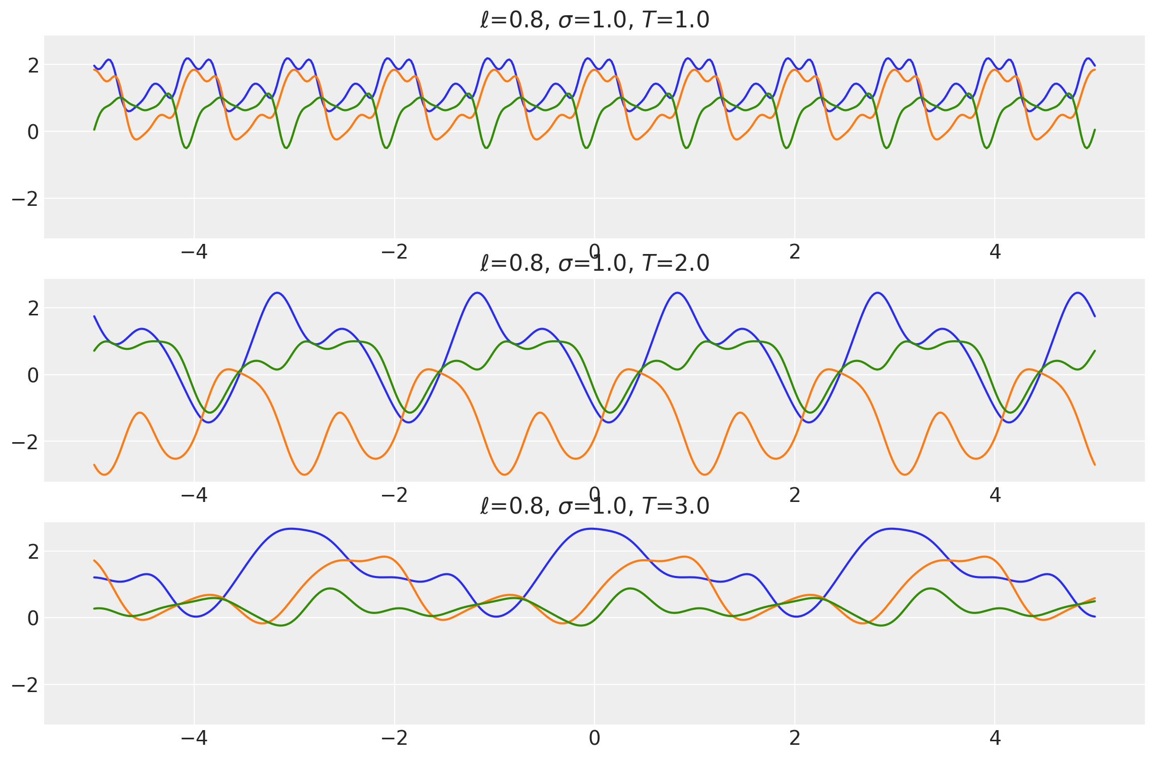
Periodic kernel aka Exponential Sine Squared Kernel comes from the Periodic Family of kernels. This kernels occilates in space with a period \(T\). This kernel is used mostly for time-series and other temporal prediction tasks. It can be expressed as:
where \(T\) is the period of the kernel.
Its signature in PyMC4 is:
k = Periodic(length_scale, amplitude=1., period=1., feature_ndims=1, active_dims=None, scale_diag=None)
length_scales = tf.constant([0.8, 0.8, 0.8], dtype=tf.float64)
amplitudes = tf.constant([1.0, 1.0, 1.0], dtype=tf.float64)
periods = tf.constant([1.0, 2.0, 3.0], dtype=tf.float64)

k = Periodic(
    length_scale=length_scales, amplitude=amplitudes, period=periods, ARD=False
)
x = np.linspace(-5, 5, num=500)[:, np.newaxis]

covs = stabilize(k(x, x), shift=1e-8)
dists = pm.MvNormal("_", loc=0.0, covariance_matrix=covs)
samples = tf.transpose(dists.sample(3), perm=[1, 0, 2])
plot_samples(
    x, samples, [length_scales, amplitudes, periods], ["$\\ell$", "$\\sigma$", "$T$"]
)
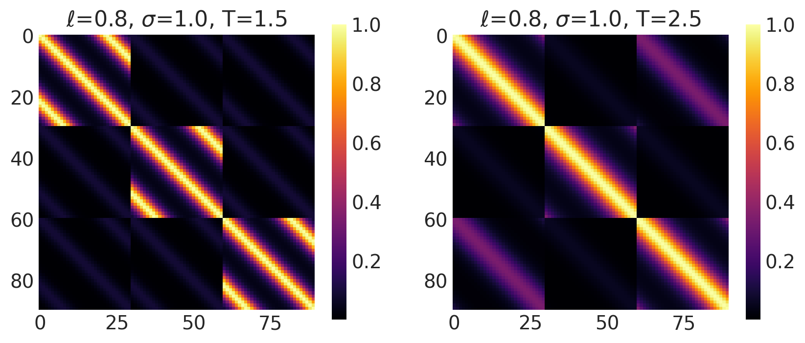
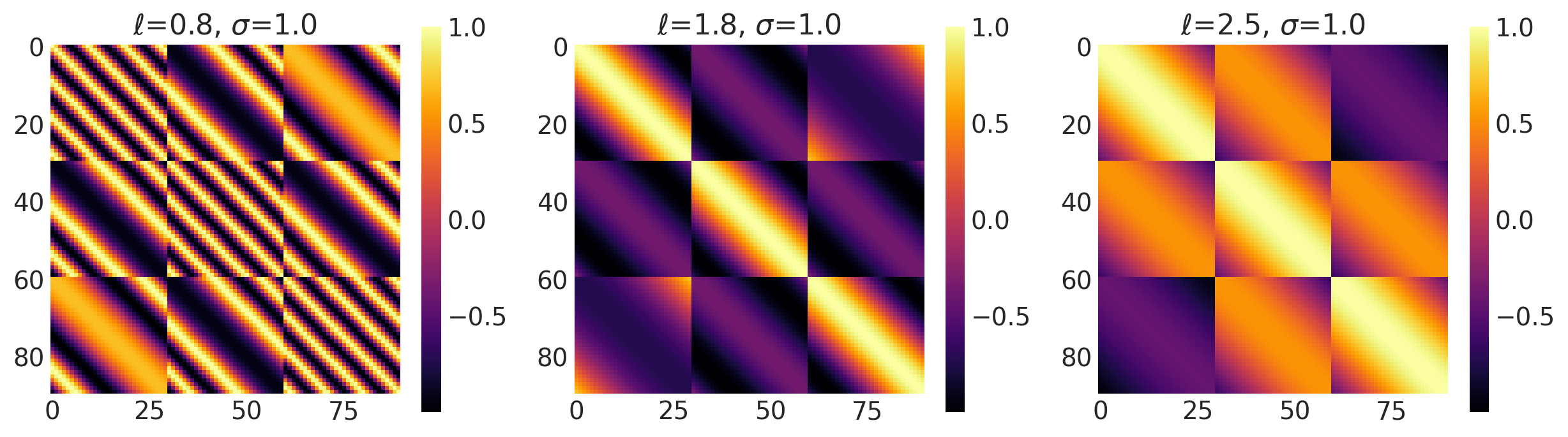
x1, x2 = np.meshgrid(np.linspace(-1, 1, 30), np.linspace(-1, 1, 3))
X2 = np.concatenate((x1.reshape(90, 1), x2.reshape(90, 1)), axis=1)

ls, amp, t = [0.8, 0.8], [1.0, 1.0], [1.5, 2.5]
k = Periodic(length_scale=ls, amplitude=amp, period=t, ARD=False)

plot_cov_matrix(k, X2, [ls, amp, t], ["$\\ell$", "$\\sigma$", "T"])
Cosine Kernel
This kernel is a part of the Periodic Kernels. It represents purely sinusoidal functions. It is given by:
Its signature in PyMC4 is:
k = Cosine(length_scale, amplitude=1., feature_ndims=1, active_dims=None, scale_diag=None)
Example 1
length_scales = tf.constant([0.4, 0.4, 0.4], dtype=tf.float64)
amplitudes = tf.constant([1.0, 5.0, 10.0], dtype=tf.float64)

k = Periodic(length_scale=length_scales, amplitude=amplitudes, ARD=False)
x = np.linspace(-5, 5, num=500)[:, np.newaxis]

covs = stabilize(k(x, x), shift=1e-8)
dists = pm.MvNormal("_", loc=0.0, covariance_matrix=covs)
samples = tf.transpose(dists.sample(3), perm=[1, 0, 2])
plot_samples(x, samples, [length_scales, amplitudes], ["$\\ell$", "$\\sigma$"])
Example 2
length_scales = tf.constant([3.4, 3.4, 3.4], dtype=tf.float64)
amplitudes = tf.constant([1.0, 5.0, 10.0], dtype=tf.float64)

k = Periodic(length_scale=length_scales, amplitude=amplitudes, ARD=False)
x = np.linspace(-5, 5, num=500)[:, np.newaxis]

covs = stabilize(k(x, x), shift=1e-8)
dists = pm.MvNormal("_", loc=0.0, covariance_matrix=covs)
samples = tf.transpose(dists.sample(3), perm=[1, 0, 2])
plot_samples(x, samples, [length_scales, amplitudes], ["$\\ell$", "$\\sigma$"])
x1, x2 = np.meshgrid(np.linspace(-1, 1, 30), np.linspace(-1, 1, 3))
X2 = np.concatenate((x1.reshape(90, 1), x2.reshape(90, 1)), axis=1)

ls, amp = [0.8, 1.8, 2.5], [1.0, 1.0, 1.0]
k = Cosine(length_scale=ls, amplitude=amp, ARD=False)

plot_cov_matrix(k, X2, [ls, amp], ["$\\ell$", "$\\sigma$"])
Non-Stationary Kernels
There are a total of 5 non-stationary distributions in PyMC4. These kernels vary not only with respect to the parameters but also with the position of data in space.
Linear Kernel
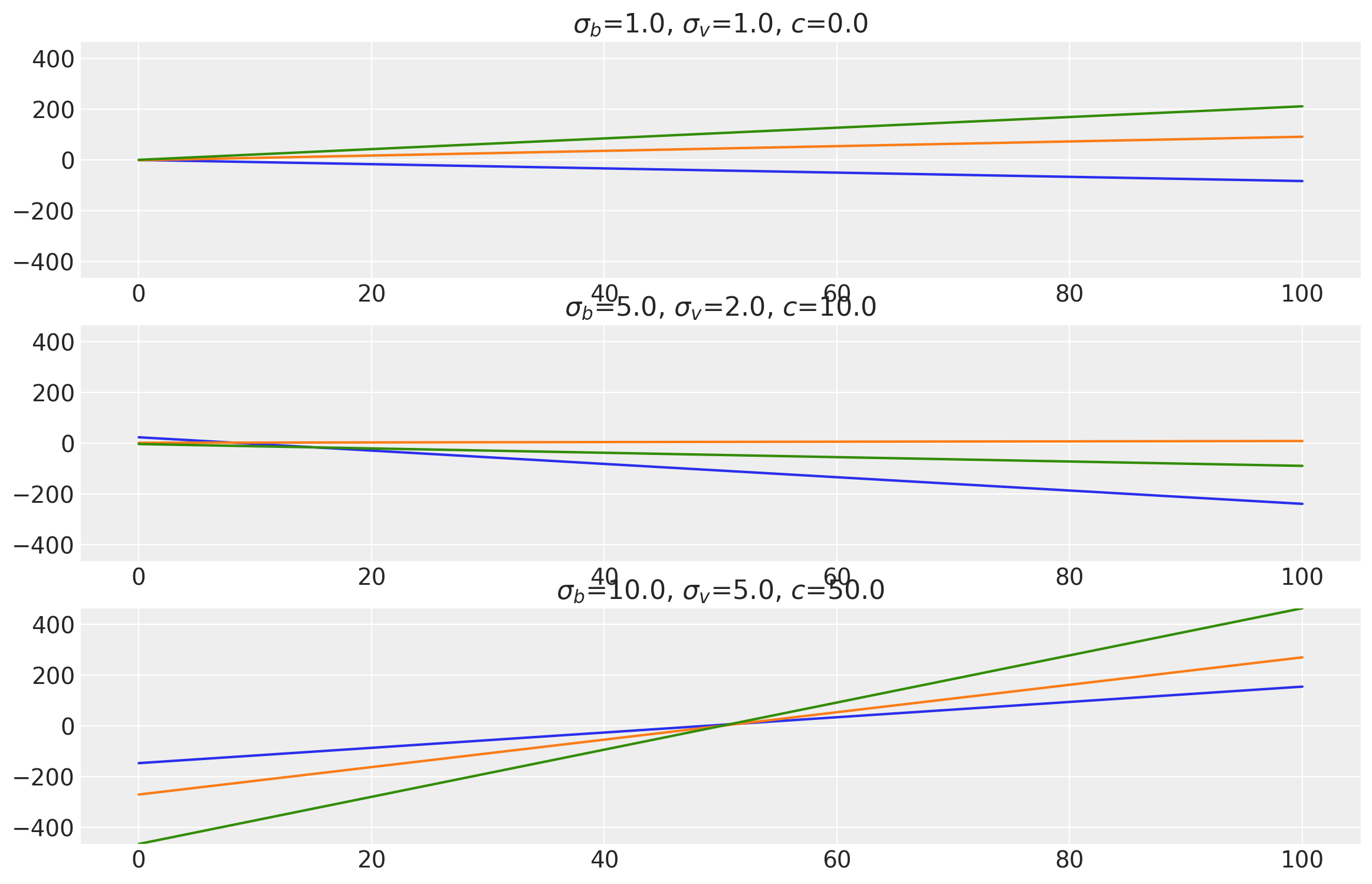
This kernel evaluates a linear function of the inputs \(x\) and \(x'\). It performs Bayesian linear regression on the inputs to produce random linear functions. The parameter \(\sigma_b\) controls how far the covariance is from the mean value and is called “bias variance”. \(\sigma_v\) controls how fast the covariance grows with respect to the origin point and is called “slope variance”. \(c\) is the shift parameter which shift points closer to the origin by \(c\) units.
where \(\sigma_b\) is bias variance, \(\sigma_v\) is slope variance, and \(c\) is the shift parameter.
Its signature in pymc4 is:
k = Linear(bias_variance, slope_variance, shift, feature_ndims=1, active_dims=None, scale_diag=None)
bias_variances = tf.constant([1.0, 5.0, 10.0], dtype=tf.float64)
slope_variances = tf.constant([1.0, 2.0, 5.0], dtype=tf.float64)
shifts = tf.constant([0.0, 10.0, 50.0], dtype=tf.float64)

k = Linear(
    bias_variance=bias_variances,
    slope_variance=slope_variances,
    shift=shifts,
    ARD=False,
)
x = np.linspace(0.0, 100.0, num=100)[:, np.newaxis]

covs = stabilize(k(x, x), shift=1e-8)
dists = pm.MvNormal("_", loc=0.0, covariance_matrix=covs)
samples = tf.transpose(dists.sample(3), perm=[1, 0, 2])
plot_samples(
    x,
    samples,
    [bias_variances, slope_variances, shifts],
    ["$\\sigma_b$", "$\\sigma_v$", "$c$"],
)
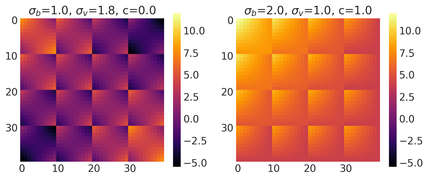
x1, x2 = np.meshgrid(np.linspace(-1, 1, 10), np.linspace(-1, 1, 4))
X2 = np.concatenate((x1.reshape(40, 1), x2.reshape(40, 1)), axis=1)

bv, sv, c = [1.0, 2.0], [1.8, 1.0], [0.0, 1.0]
k = Linear(bias_variance=bv, slope_variance=sv, shift=c, ARD=False)

plot_cov_matrix(k, X2, [bv, sv, c], ["$\\sigma_b$", "$\\sigma_v$", "c"])
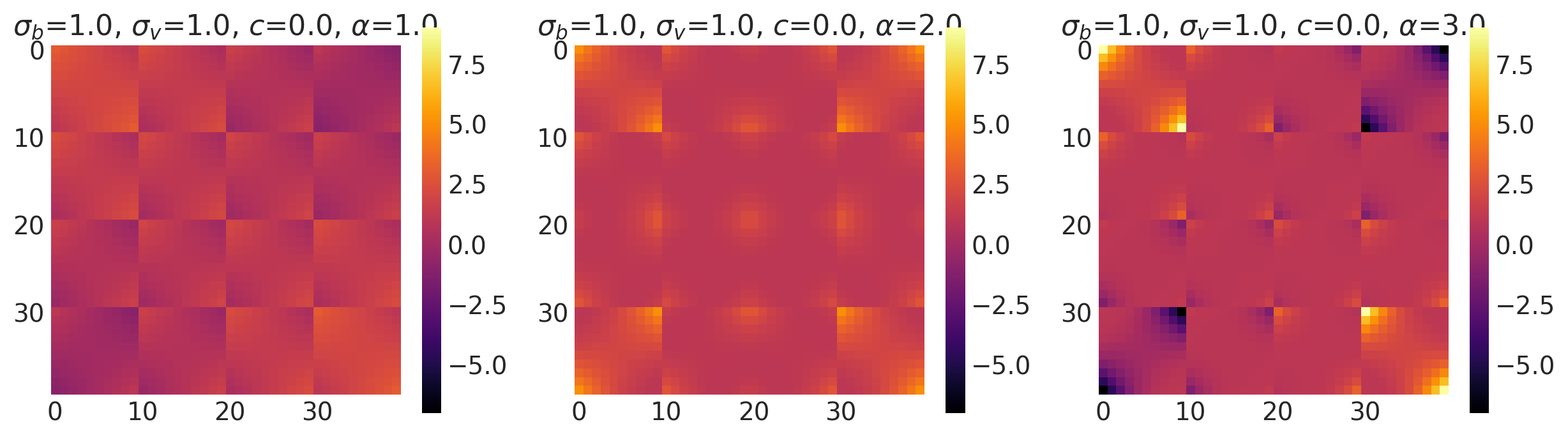
Polynomial Kernel
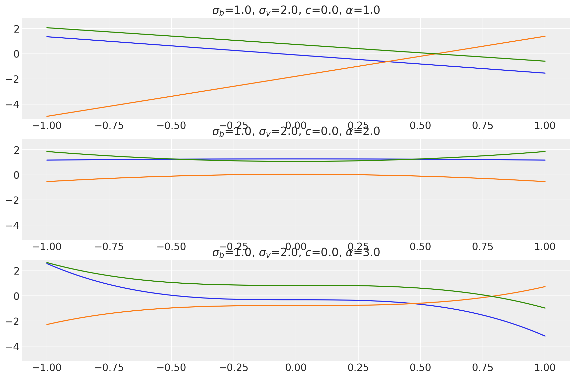
This kernel is a generalization over the Linear Kernel and performs polynomial regression on the data to evaluate the covariance matrix. An extra parameter \(\alpha\) controls the degree of the polynomial. This kernel is exactly the same as the Linear Kernel when \(\alpha=1\).
This kernel can be represented mathematically as:
where \(\sigma_b\), \(\sigma_v\) and \(c\) are the same as before and \(\alpha\) is the exponent.
Its signature in pymc4 is:
k = Polynomial(bias_variance, slope_variance, shift, exponent, feature_ndims=1, active_dims=None, scale_diag=None)
bias_variances = tf.constant([1.0] * 3, dtype=tf.float64)
slope_variances = tf.constant([2.0] * 3, dtype=tf.float64)
shifts = tf.constant([0.0] * 3, dtype=tf.float64)
exponents = tf.constant([1.0, 2.0, 3.0], dtype=tf.float64)

k = Polynomial(
    bias_variance=bias_variances,
    slope_variance=slope_variances,
    shift=shifts,
    exponent=exponents,
    ARD=False,
)
x = np.linspace(-1.0, 1.0, num=100)[:, np.newaxis]

covs = stabilize(k(x, x), shift=1e-8)
dists = pm.MvNormal("_", loc=0.0, covariance_matrix=covs)
samples = tf.transpose(dists.sample(3), perm=[1, 0, 2])
plot_samples(
    x,
    samples,
    [bias_variances, slope_variances, shifts, exponents],
    ["$\\sigma_b$", "$\\sigma_v$", "$c$", "$\\alpha$"],
)
x1, x2 = np.meshgrid(np.linspace(-1, 1, 10), np.linspace(-1, 1, 4))
X2 = np.concatenate((x1.reshape(40, 1), x2.reshape(40, 1)), axis=1)

bv, sv, c, e = [1.0, 1.0, 1.0], [1.0, 1.0, 1.0], [0.0, 0.0, 0.0], [1.0, 2.0, 3.0]
k = Polynomial(bias_variance=bv, slope_variance=sv, shift=c, exponent=e, ARD=False)

plot_cov_matrix(
    k, X2, [bv, sv, c, e], ["$\\sigma_b$", "$\\sigma_v$", "$c$", "$\\alpha$"]
)
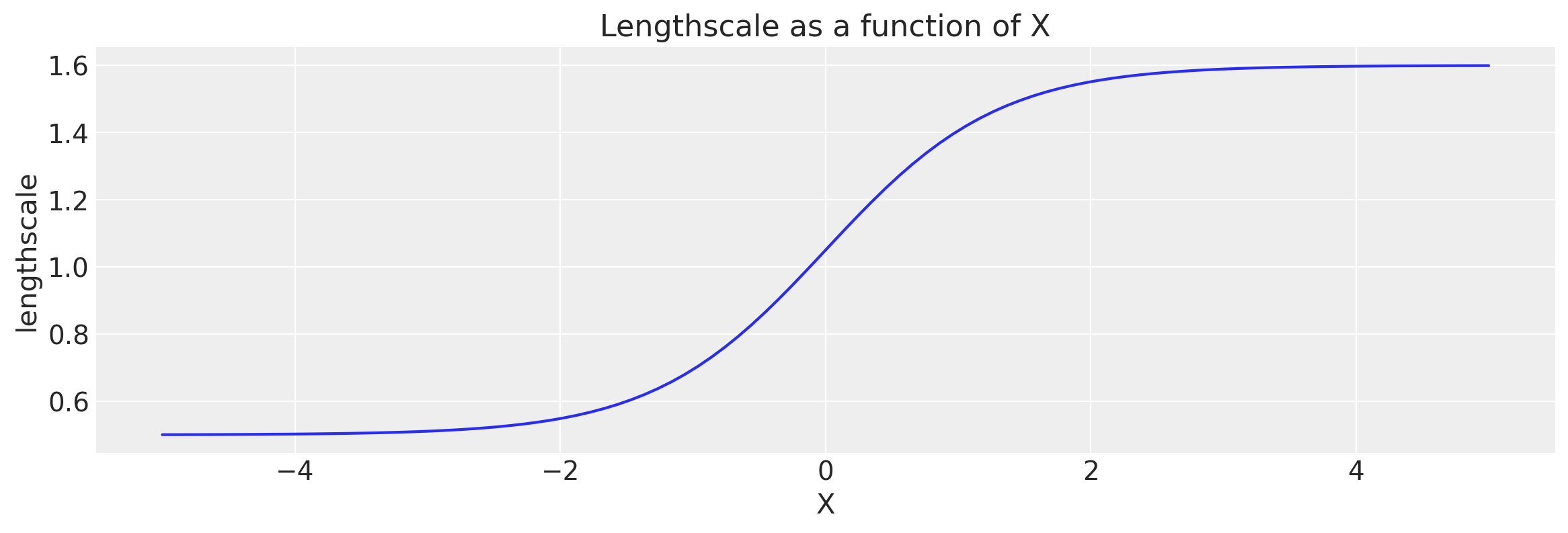
Gibbs Kernel
This kernel comes from a non-stationary family of kernels. The length_scale parameter varies with varying inputs. It is expressed as:
where \(\ell(.)\) is a function of inputs that outputs a different length scale for each of the input points.
The signature of this kernel in PyMC4 is
k = Gibbs(length_scale_fn, fn_args, feature_ndims=1, active_dims=None, scale_diag=None)
This kernel expects length_scale_fn to have the following signature:
def length_scale_fn(x: array_like, *fn_args) -> array_like:
    ...
The array_like type can be any type of array (numpy array, tensorflow tensor, etc) of the same shape as the input where each entry corresponds to the length_scale for that point.
Notes
This kernel is very slow and computationally heavy compared to other kernels. It works best with inputs having a single feature dimension and a single entry in that dimension. This means the inputs should have the shape (..., n, 1) and (..., m, 1). Other inputs will work but the evaluation will be very slow.
No argument validation is done even when validate_args=True.
def tanh_fn(x, ls1, ls2, w, x0):
    """
    ls1: left saturation value
    ls2: right saturation value
    w:   transition width
    x0:  transition location.
    """
    return (ls1 + ls2) / 2 - (ls1 - ls2) / 2 * tf.tanh((x - x0) / w)


ls1 = tf.constant(0.5, dtype=tf.float64)
ls2 = tf.constant(1.6, dtype=tf.float64)
w = tf.constant(1.3, dtype=tf.float64)
x0 = tf.constant(0.0, dtype=tf.float64)
# You can also partial the length_scale function to avoid passing extra argumets.
# from functools import partial
# fn = partial(tanh_fn, ls1=ls1, ls2=ls2, w=w, x0=x0)
k = Gibbs(
    length_scale_fn=tanh_fn, fn_args=(ls1, ls2, w, x0), dtype=tf.float64, ARD=False
)
# Let's visualize the tanh function
x = np.linspace(-5.0, 5.0, num=100)[:, np.newaxis]

wf = tanh_fn(x, ls1, ls2, w, x0)
plt.figure(figsize=(14, 4))
plt.plot(x, wf)
plt.ylabel("lengthscale")
plt.xlabel("X")
plt.title("Lengthscale as a function of X");
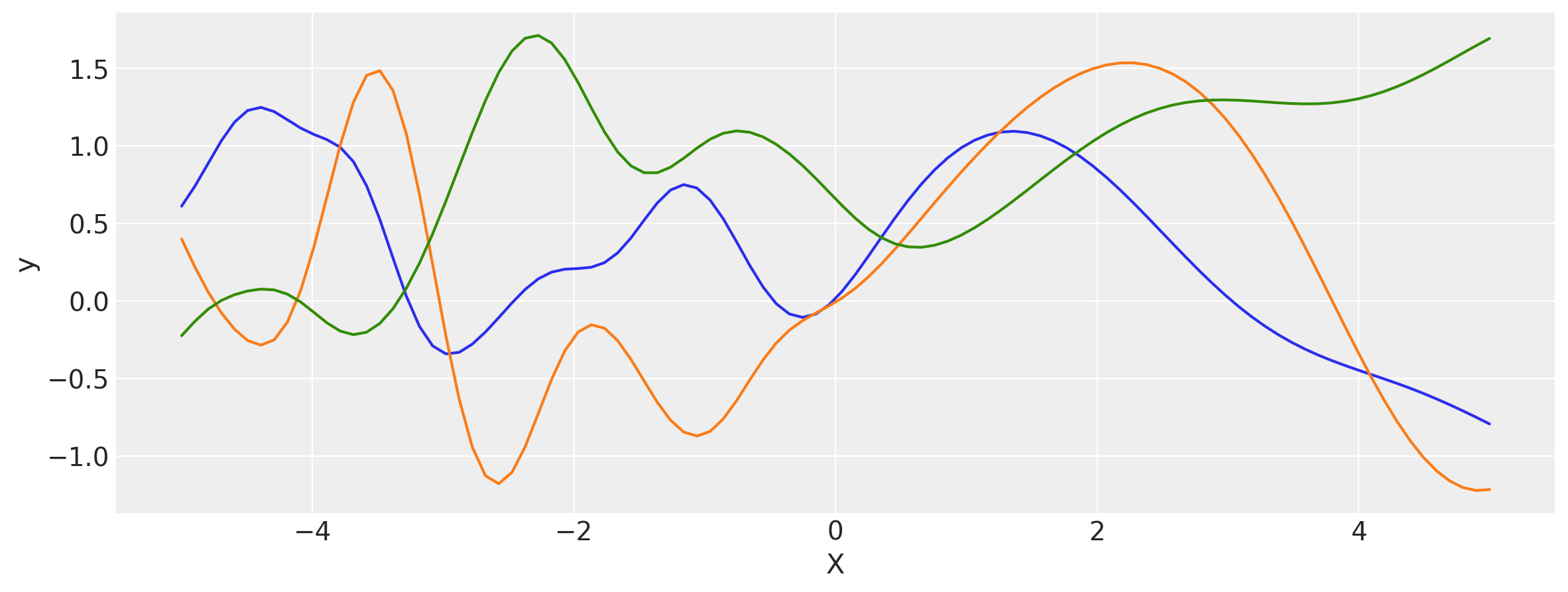
# Let's evaluate the covariance matrix.
covs = stabilize(k(x, x), shift=1e-8)
dists = pm.MvNormal("_", loc=0, covariance_matrix=covs)
samples = dists.sample(3)
plt.figure(figsize=(14, 5))
[plt.plot(x, samples[i, :]) for i in range(3)]
plt.xlabel("X")
plt.ylabel("y")
plt.show()
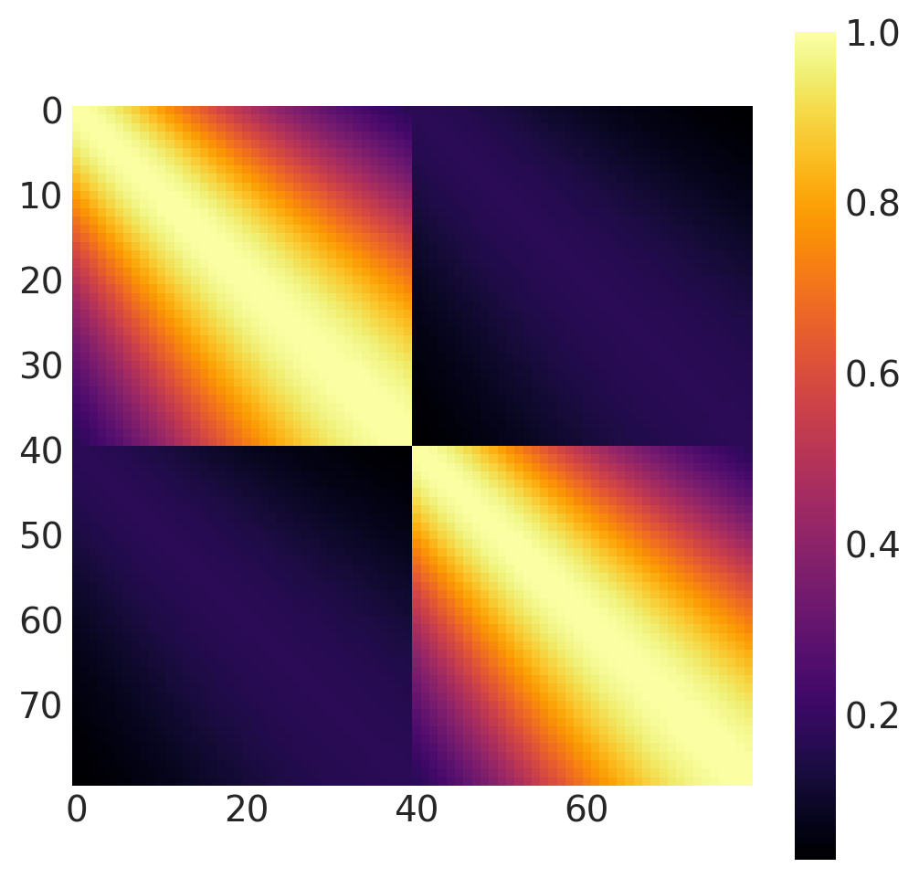
x1, x2 = np.meshgrid(np.linspace(-1, 1, 40), np.linspace(-1, 1, 2))
X2 = np.concatenate((x1.reshape(80, 1), x2.reshape(80, 1)), axis=1)

k = Gibbs(
    length_scale_fn=tanh_fn, fn_args=(ls1, ls2, w, x0), dtype=tf.float64, ARD=False
)

cov = k(X2, X2)
plt.figure(figsize=(6, 6))
m = plt.imshow(cov, cmap="inferno", interpolation="none")
plt.grid(False)
plt.colorbar(m);
Scaled Covariance Kernel
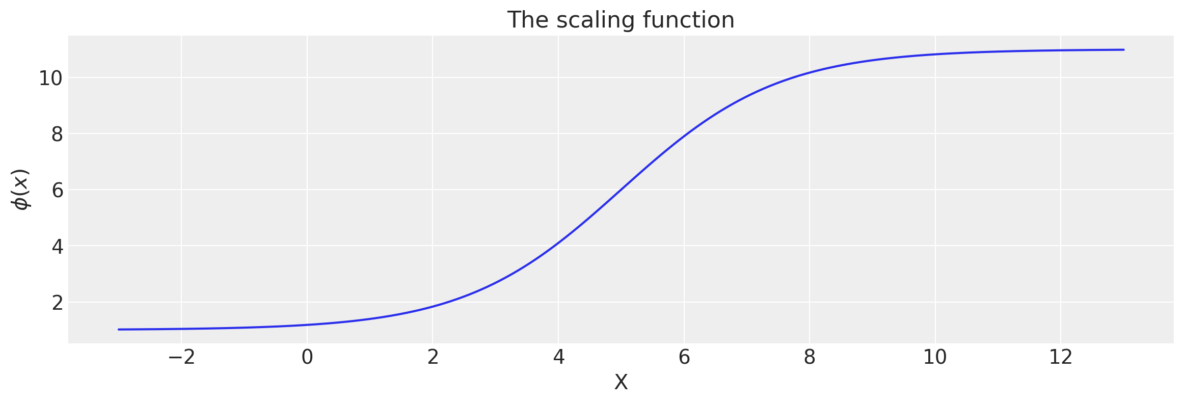
This kernel uses a scaling function to scale the covariance between two points evaluated using some other kernel. This scaling function is a function of the inputs and returns an output of the same shape. It can be expressed as
where \(k(x,x')\) is the kernel function used to evaluate the covariance matrix and \(f(x, \theta)\) is the scaling function of the inputs \(x\) and some \(\theta\) that can be inferred during sampling/inference.
Its signature in PyMC4 is
k = ScaledCov(kernel, scaling_fn, fn_args=None)
This kernel expects the function scaling_fn to have a signature
def scaling_fn(x: array_like, *fn_args) -> array_like:
    ...
It must return an array of the same shape as that of the input x.
Notes
This kernel doesn’t perform argument validation even when validate_args=True.
def logistic(x, a, x0, c, d):
    # a is the slope, x0 is the location
    # d is the coefficient of the sigmoid term
    # c is the bias of the linear equation
    return d * tf.sigmoid(a * (x - x0)) + c


a = tf.constant(0.8, dtype=tf.float64)
x0 = tf.constant(5.0, dtype=tf.float64)
c = tf.constant(1.0, dtype=tf.float64)
d = tf.constant(10.0, dtype=tf.float64)

kernel = ExpQuad(tf.constant(0.2, dtype=tf.float64), ARD=False)
k = ScaledCov(kernel=kernel, scaling_fn=logistic, fn_args=(a, x0, c, d), ARD=False)
# Let's visualize the logistic function.
x = np.linspace(-3.0, 13.0, 500)[:, None]
lfunc = logistic(x, a, x0, c, d)

plt.figure(figsize=(14, 4))
plt.plot(x, lfunc)
plt.xlabel("X")
plt.ylabel("$\phi(x)$")
plt.title("The scaling function");
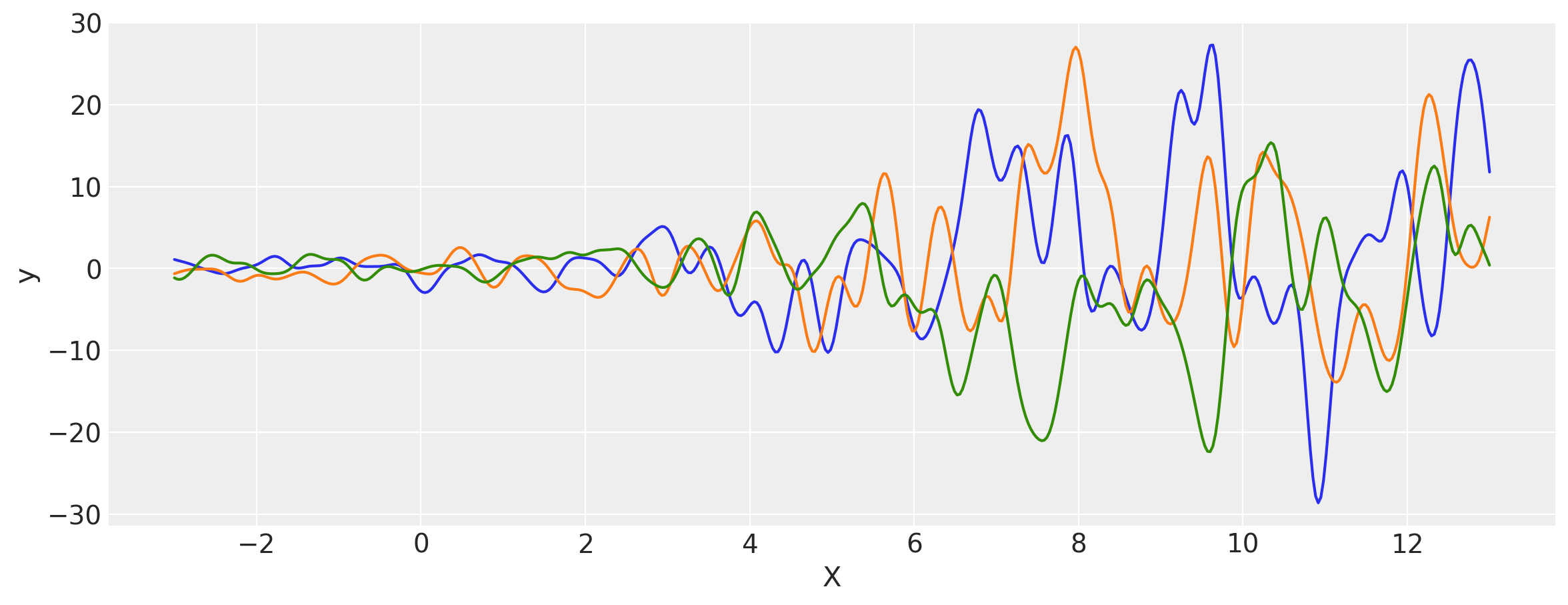
# Let's evaluate the covariance matrix.
covs = stabilize(k(x, x), shift=1e-8)
dists = pm.MvNormal("_", loc=0, covariance_matrix=covs)
samples = dists.sample(3)
plt.figure(figsize=(14, 5))
[plt.plot(x, samples[i, :]) for i in range(3)]
plt.xlabel("X")
plt.ylabel("y")
plt.show()
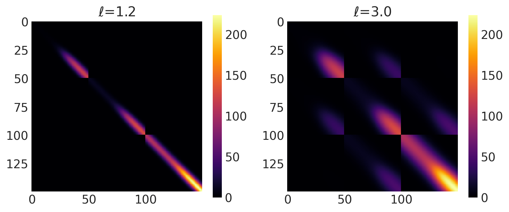
x1, x2 = np.meshgrid(np.linspace(-4, 12, 50), np.linspace(-1, 8, 3))
X2 = np.concatenate((x1.reshape(150, 1), x2.reshape(150, 1)), axis=1)

ls = [1.2, 3.0]
kernel = ExpQuad(tf.constant(ls, dtype=tf.float64), ARD=False)
k = ScaledCov(kernel=kernel, scaling_fn=logistic, fn_args=(a, x0, c, d), ARD=False)

plot_cov_matrix(k, X2, [ls], ["$\\ell$"])
Warped Input Kernel
This kernel transforms the input using a transformation function and uses it instead to evaluate the covariance matrix. This is also called FeatureTransformed kernel. It’s mathematical form is
where \(f(.)\) is a warping (transformation) function.
Its signature in PyMC4 is
k = WarpedInput(kernel, warp_fn, fn_args=None)
It expects the signature of function warp_fn to be:
def warp_fn(x: array_like, *fn_args) -> array_like:
    ...
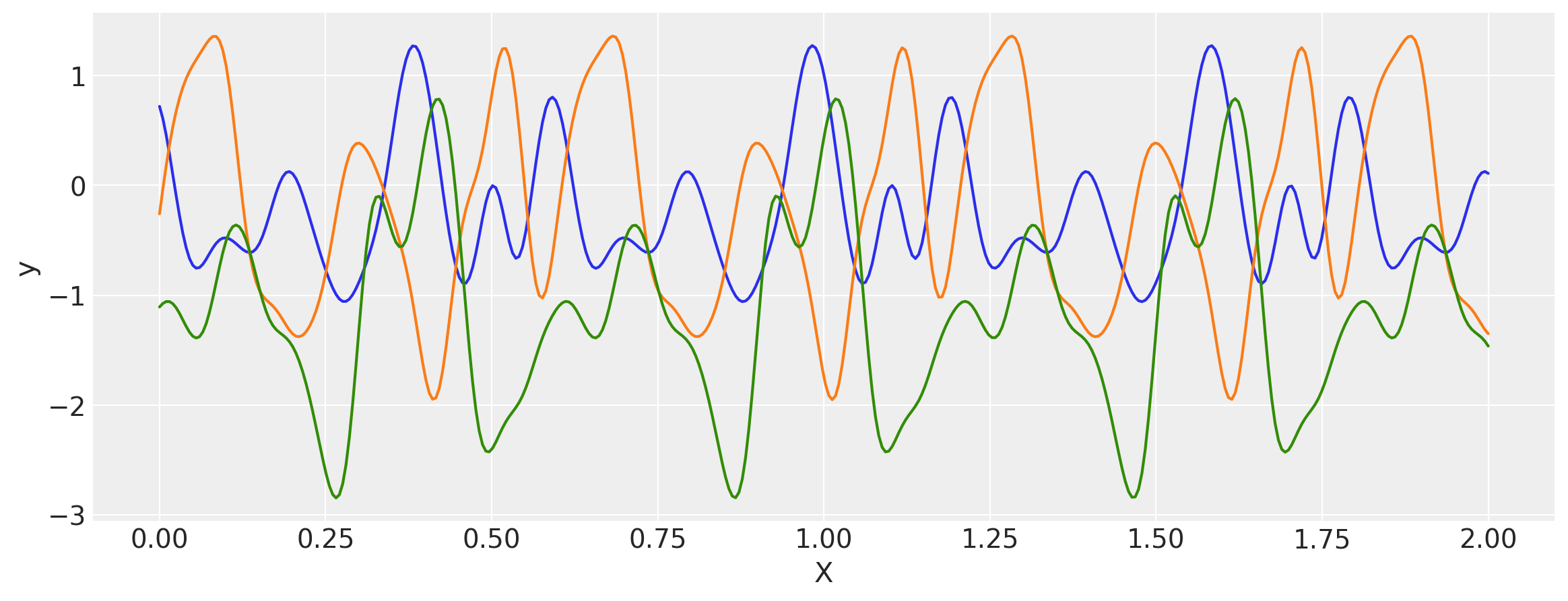
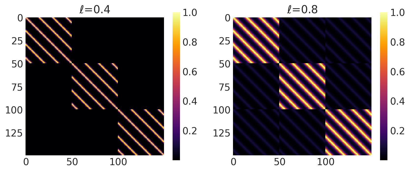
Below is an example of constructing a Periodic kernel using the warped input kernel!
Notes
This kernel doesn’t perform argument validation even if validate_args=True.
def mapping(x, T):
    c = 2.0 * np.pi * (1.0 / T)
    u = tf.concat((tf.math.sin(c * x), tf.math.cos(c * x)), axis=1)
    return u


T = tf.constant(0.6, dtype=tf.float64)
ls = tf.constant(0.4, dtype=tf.float64)

kernel = ExpQuad(ls, ARD=False)
k = WarpedInput(kernel=kernel, warp_fn=mapping, fn_args=(T,), ARD=False)
x = np.linspace(0, 2, 400)[:, None]
covs = stabilize(k(x, x), shift=1e-8)
dists = pm.MvNormal("_", loc=0, covariance_matrix=covs)
samples = dists.sample(3)
plt.figure(figsize=(14, 5))
[plt.plot(x, samples[i, :]) for i in range(3)]
plt.xlabel("X")
plt.ylabel("y")
plt.show()
x1, x2 = np.meshgrid(np.linspace(-1, 1, 50), np.linspace(-1, 1, 3))
X2 = np.concatenate((x1.reshape(150, 1), x2.reshape(150, 1)), axis=1)

ls = tf.constant([0.4, 0.8], dtype=tf.float64)
kernel = ExpQuad(ls, ARD=False)
k = WarpedInput(kernel=kernel, warp_fn=mapping, fn_args=(T,), ARD=False)

plot_cov_matrix(k, X2, [ls], ["$\\ell$"])
Combinations of Kernel
PyMC4 allows combinations of kernels to generate new kernels. This can be very helpful to construct new kernels that aren’t directly imlemented in PyMC4. This includes
This section shows how to use both addition and multiplication on kernels.
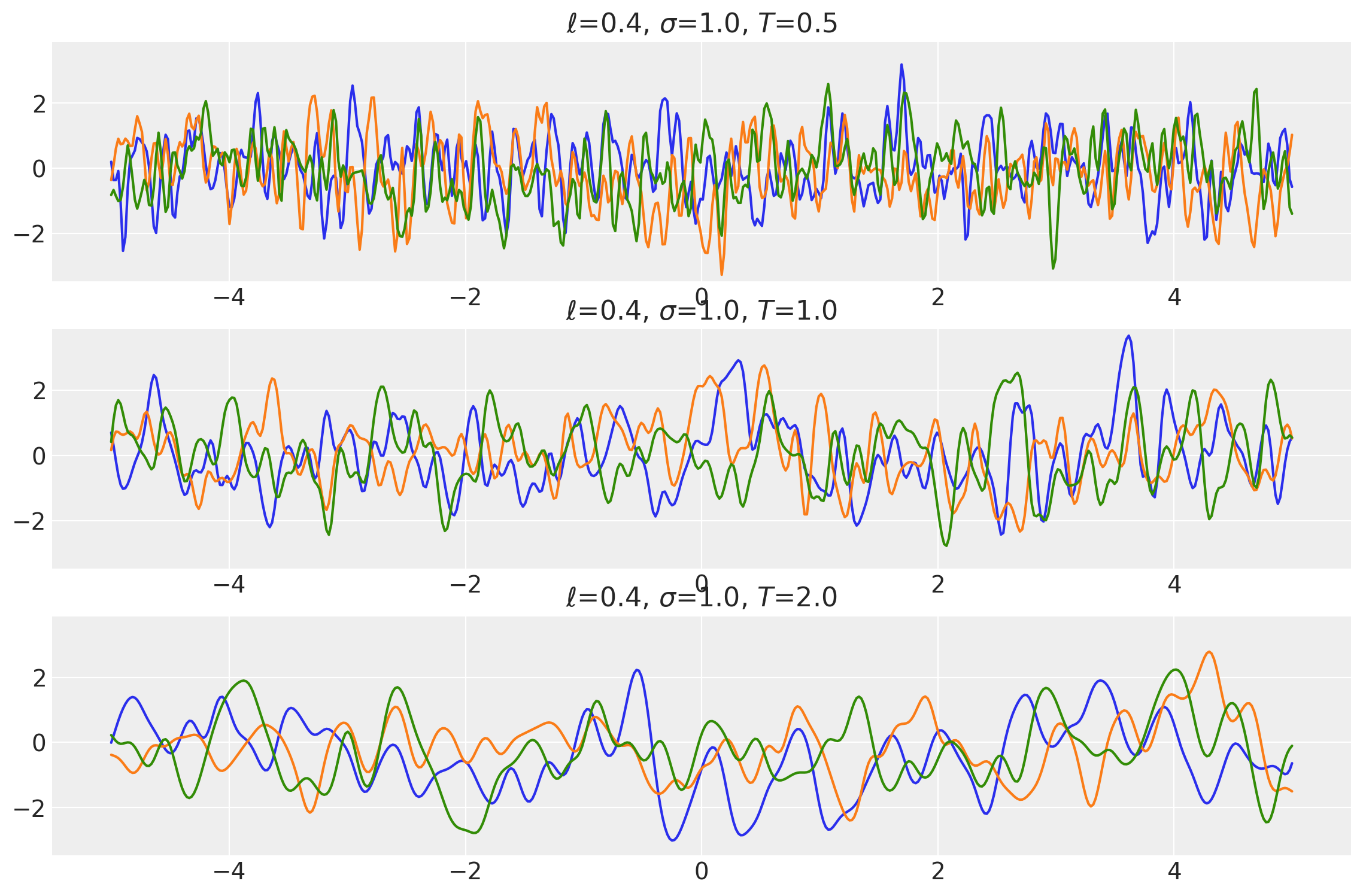
Locally Periodic Kernel
Locally Periodic kernel is a product of the ExpQuad and periodic kernel. Its mathematical formula is
It can be impemented in PyMC4 using the product * operator.
k = ExpQuad(length_scale, amplitude, ...) * Periodic(length_scale, amplitude, period, ...)
This new kernel k has all the methods that other covariance functions have.
Example 1
ls = tf.constant([0.4, 0.4, 0.4], dtype=tf.float64)
amp = tf.constant([1.0, 1.0, 1.0], dtype=tf.float64)

k1 = ExpQuad(length_scale=ls, amplitude=amp, ARD=False)

periods = tf.constant([0.5, 1.0, 2.0], dtype=tf.float64)

k2 = Periodic(length_scale=ls, amplitude=amp, period=periods, ARD=False)

k = k1 * k2
x = np.linspace(-5, 5, num=500)[:, np.newaxis]

covs = stabilize(k(x, x), shift=1e-8)
dists = pm.MvNormal("_", loc=0.0, covariance_matrix=covs)
samples = tf.transpose(dists.sample(3), perm=[1, 0, 2])
plot_samples(x, samples, [ls, amp, periods], ["$\\ell$", "$\\sigma$", "$T$"])
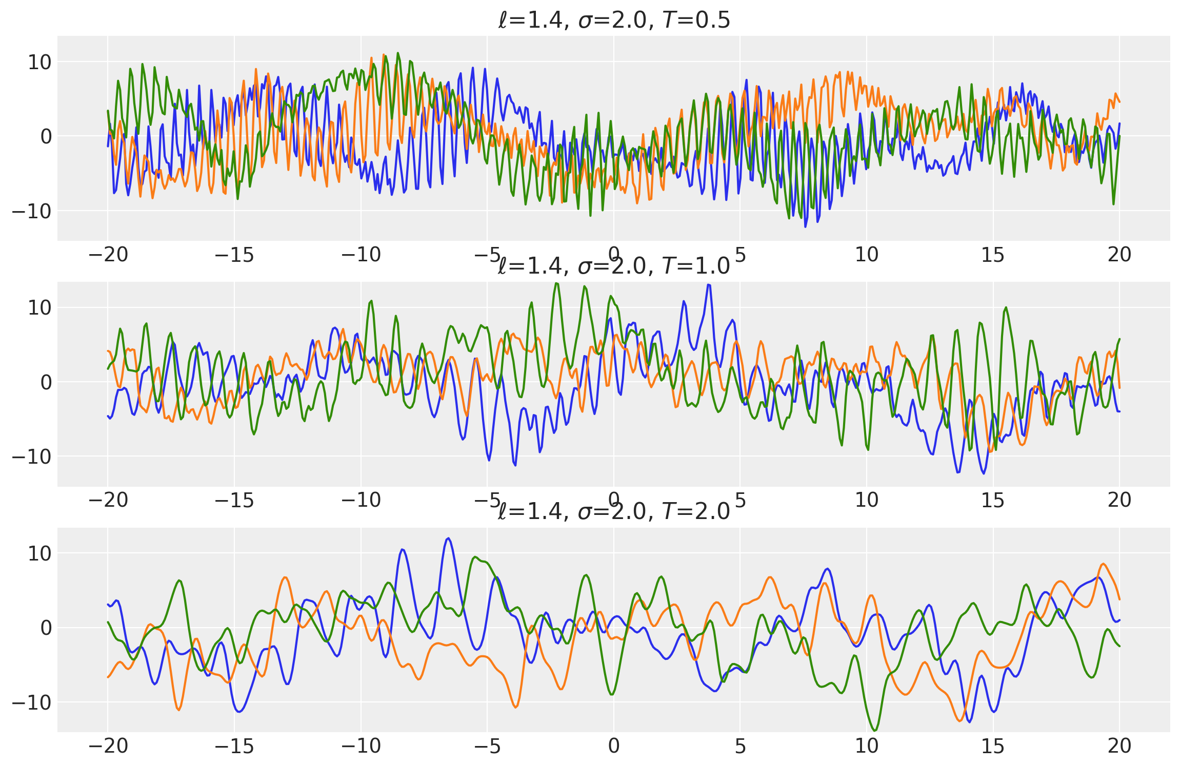
Example 2
ls = tf.constant([1.4, 1.4, 1.4], dtype=tf.float64)
amp = tf.constant([2.0, 2.0, 2.0], dtype=tf.float64)

k1 = ExpQuad(length_scale=ls, amplitude=amp, ARD=False)

periods = tf.constant([0.5, 1.0, 2.0], dtype=tf.float64)

k2 = Periodic(length_scale=ls, amplitude=amp, period=periods, ARD=False)

k = k1 * k2
x = np.linspace(-20, 20, num=500)[:, np.newaxis]

covs = stabilize(k(x, x), shift=1e-8)
dists = pm.MvNormal("_", loc=0.0, covariance_matrix=covs)
samples = tf.transpose(dists.sample(3), perm=[1, 0, 2])
plot_samples(x, samples, [ls, amp, periods], ["$\\ell$", "$\\sigma$", "$T$"])
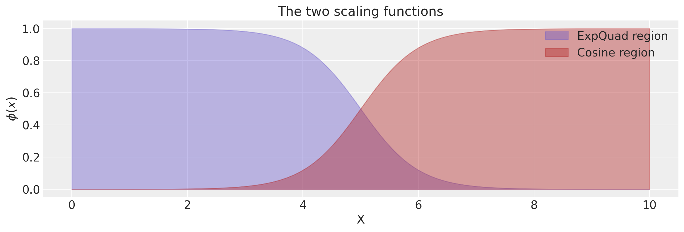
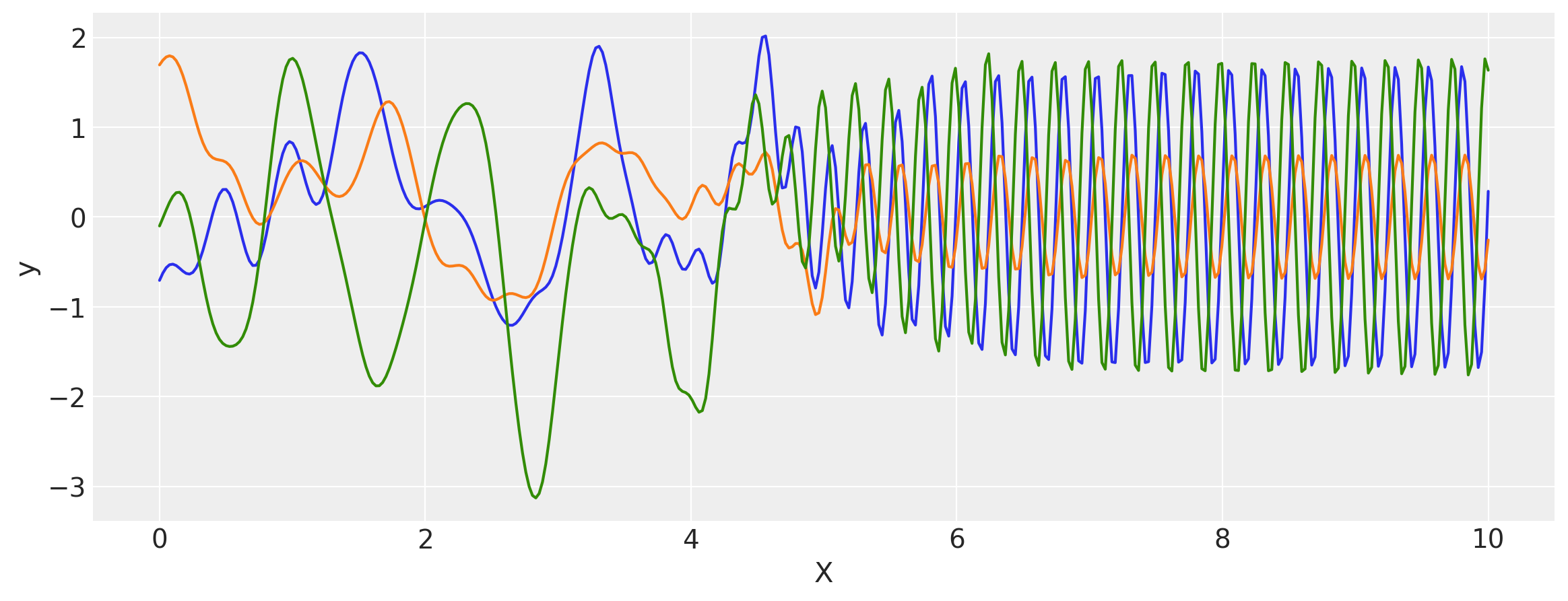
Changepoint Kernel
The ScaledCov kernel can be used to create the Changepoint covariance. This covariance models a process that gradually transitions from one type of behavior to another.
The changepoint kernel is given by
def logistic(x, a, x0):
    # a is the slope, x0 is the location
    return tf.sigmoid(a * (x - x0))


a = tf.constant(2.0, dtype=tf.float64)
x0 = tf.constant(5.0, dtype=tf.float64)

k1 = ScaledCov(
    kernel=ExpQuad(np.array(0.2), ARD=False),
    scaling_fn=logistic,
    fn_args=(-a, x0),
    ARD=False,
)
k2 = ScaledCov(
    kernel=Cosine(np.array(0.5), ARD=False),
    scaling_fn=logistic,
    fn_args=(a, x0),
    ARD=False,
)
k = k1 + k2
x = np.linspace(0, 10, 400)
plt.figure(figsize=(14, 4))
plt.fill_between(
    x,
    np.zeros(400),
    logistic(x, -a, x0),
    label="ExpQuad region",
    color="slateblue",
    alpha=0.4,
)
plt.fill_between(
    x,
    np.zeros(400),
    logistic(x, a, x0),
    label="Cosine region",
    color="firebrick",
    alpha=0.4,
)
plt.legend()
plt.xlabel("X")
plt.ylabel("$\phi(x)$")
plt.title("The two scaling functions");
covs = stabilize(k(x[:, None], x[:, None]), shift=1e-8)
dists = pm.MvNormal("_", loc=0.0, covariance_matrix=covs)
samples = dists.sample(3)
plt.figure(figsize=(14, 5))
[plt.plot(x, samples[i, :]) for i in range(3)]
plt.xlabel("X")
plt.ylabel("y")
plt.show()
%load_ext watermark
%watermark -n -u -v -iv -w
pymc4      4.0a2
numpy      1.18.5
tensorflow 2.3.0-dev20200608
arviz      0.8.3
last updated: Thu Jul 02 2020

CPython 3.7.3
IPython 7.15.0
watermark 2.0.2