Marginal Gaussian Process
The Model
A Marginal Gaussian process jointly represents the data as a large probability distribution. This distribution, as we will see, turns out to a normal distribution in classical Bayesian approaches. Suppose we have some data \(X, y\) using which we want to predict the distribution over some \(y_*\) given new data \(X_*\). We write this as:
This distribution is known as the conditional distribution.
We can construct this joint density through the use of the following decomposition:
where we represent all the parameters by \(\theta\) and \(P(\theta \mid X, y)\) is the posterior density given data and \(P(y_* \mid X_*, \theta)\) is known as the marginal likelihood of the individual test point given the parameters.
The marginal likelihood of the model is assumed to be a gaussian with parameters:
where \(m(\cdot)\) is the mean function and \(K(\cdot)\) is the kernel function. The mean function evaluates a mean vector. The kernel function takes some parameters \(\theta\), evaluates the covariance between every pair of data points, and outputs a covariance matrix. The \(\delta(\cdot)\) is the Kronecker delta function and \(\epsilon\) is a small noise. The delta function adds a small noise corruption and is equivalent to adding noise distributed as \(\mathcal{N}(0, \epsilon\mathrm{I})\).
This mean vector and the covariance matrix is then input to the multivariate normal distribution. This choice of using a normal distribution makes the integral in the conditional distribution analytical, hence, making it easy to infer a distribution over the test data for prediction and generation.
Performing Inference
The conditional distribution can also be shown to be a normal distribution with parameters:
where
This distribution can be used to make predictions over the test data or generate predictive samples.
References
- http://www.cs.cornell.edu/courses/cs4780/2017sp/lectures/lecturenote15.html
- http://inverseprobability.com/talks/notes/gaussian-processes.html
MarginalGP Model
MarginalGP model is the implementation of the Marginal GP model in PyMC4. It contains marginal_likelihood and conditional method that does exactly as described in the previous section. Moreover, it also has methods predict and predictt to sample from the conditional distribution and to get point estimate (\(\mu_{y_* \mid D}\)) of the conditional distribution respectively.
Let’s see each method in detail in the following sections:
marginal_likelihood method
First, we need to instantiate the model using a kernel function and (optionally) a mean function.
from pymc4.gp import MarginalGP
from pymc4.gp.cov import ExpQuad

# Let's first instantiate a kernel
K = ExpQuad(length_scale = 1.)

# Now, we can instantiata the model
gp = MarginalGP(cov_fn = K)
Now, To get the marginal_likelihood of the MarginalGP over some data X (of shape (n_samples, n_features)) with labels y (of shape (n_samples, )), use:
noise = 1e-2
y_ = gp.marginal_likelihood("y_", X, y, noise=noise)
You can also pass a covariance object as noise to the marginal_likelihood
method:
# kronecker delta function with epsilon 1e-2
noise = WhiteNoise(1e-2)
y_ = gp.marginal_likelihood("y_", X, y, noise=noise)
If y is not the observed data, pass is_observed=False in the
marginal likelihood method:
y_ = gp.marginal_likelihood("y_", X, y, noise=noise, is_observed=False)
By default, some jitter is added to ensure Cholesky Decomposition passes.
This behavior can be turned off by passing jitter=0 in the marginal
likelihood method:
y_ = gp.marginal_likelihood("y_", X, y, noise=noise, jitter=0)
As noise behaves exactly as jitter, it is recommended to set jitter=False
to avoid adding extra noise.
conditional method
You can use conditional method to get the conditional distribution over the new data points. This distribution can be used to predict over the new data points:
y_pred = gp.conditional("y_pred", Xnew, given={"X": X, "y": y, "noise": noise})
where Xnew are the test points (new data points) and y_pred is a multivariate normal distribution. given dictionary is optional when marginal_likelihood method has been called before.
y_ = gp.marginal_likelihood("y_", X, y, noise=noise)
y_pred = gp.conditional("y_pred", Xnew) # no need to pass given
To add noise in the conditional distribution, use:
y_pred = gp.conditional("y_pred", Xnew, pred_noise=True)
To avoid reparametrizing to the MvNormalCholesky distribution, use:
y_pred = gp.conditional("y_pred", Xnew, reparametrize=False)
Notes
The data and the parameters must have the same datatype. For example, if the data is represented as float64 then all the parameters must also be represented as float64 datatype only. Using different datatypes in-between the model will raise an exception.
import arviz as az
import matplotlib.pyplot as plt
import numpy as np
import pymc4 as pm
from pymc4.gp import MarginalGP
from pymc4.gp.cov import ExpQuad
from sklearn.decomposition import KernelPCA
from sklearn import datasets
from sklearn.preprocessing import StandardScaler
import tensorflow as tf
%config InlineBackend.figure_format = 'retina'
RANDOM_SEED = 8927
np.random.seed(RANDOM_SEED)
tf.random.set_seed(RANDOM_SEED)
az.style.use('arviz-darkgrid')
Example 1 : GP-LVM using a Linear Kernel
Marginal Gaussian Processes can be used to perform Principal Component Analysis (PCA) (a technique to project and visualize high dimensional data onto a low dimensional feature space) using a model called Gaussian Process Latent Variable Model (GP-LVM). GP-LVMs generally outperform the native PCS algorithm and can even generalize further using non-linear kernel functions like RBF kernel. This property of GP-LVMs makes them more auspicious over vanilla PCA. To learn more about GP-LVMs, refer [1].
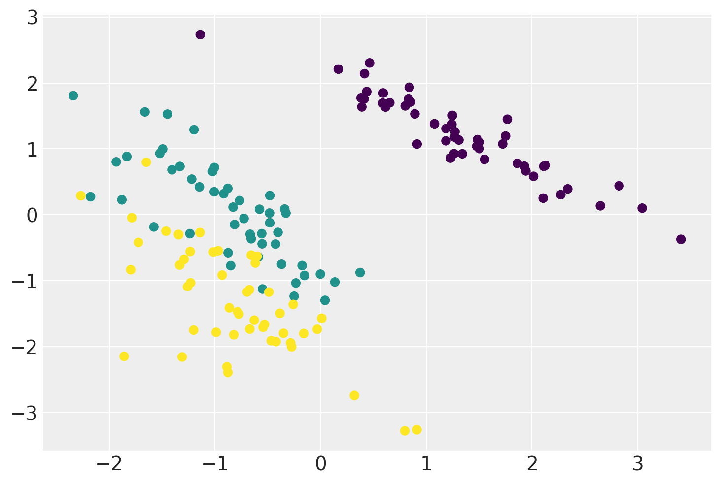
Below is an example of a Linear GP-LVM that projects the Iris Flower Dataset onto two-dimensional feature space while preserving a clear separation between different types of flowers.
References
[1] Neil D. Lawrence, 2003, Gaussian process latent variable models for visualization of high dimensional data, https://papers.nips.cc/paper/2540-gaussian-process-latent-variable-models-for-visualisation-of-high-dimensional-data.pdf
# Load the data. Needs sklearn - Use `pip install sklearn` inside the python
# environment/conda prompt/terminal to install sklearn locally.

iris = datasets.load_iris()
Y = StandardScaler().fit_transform(iris.data)

N, P = Y.shape
# Linear GP-LVM model
@pm.model
def GPLVM():
# A normal prior over the projected data
x = yield pm.MvNormalCholesky('x', loc=np.zeros(2), scale_tril=np.eye(2), batch_stack=N)
# Prior over the argumemnts of the covariance function.
args = yield pm.HalfCauchy('args', np.array(5.), batch_stack=3)
cov_fn = pm.gp.cov.Linear(args[0], args[1], args[2])
gp = pm.gp.MarginalGP(cov_fn=cov_fn)
# We put a marginal likelihood over every feature in the dataset.
for i in range(4):
y = yield gp.marginal_likelihood(f'y{i}', X=x, y=Y[:, i], noise=np.array(0.01))
model = GPLVM()
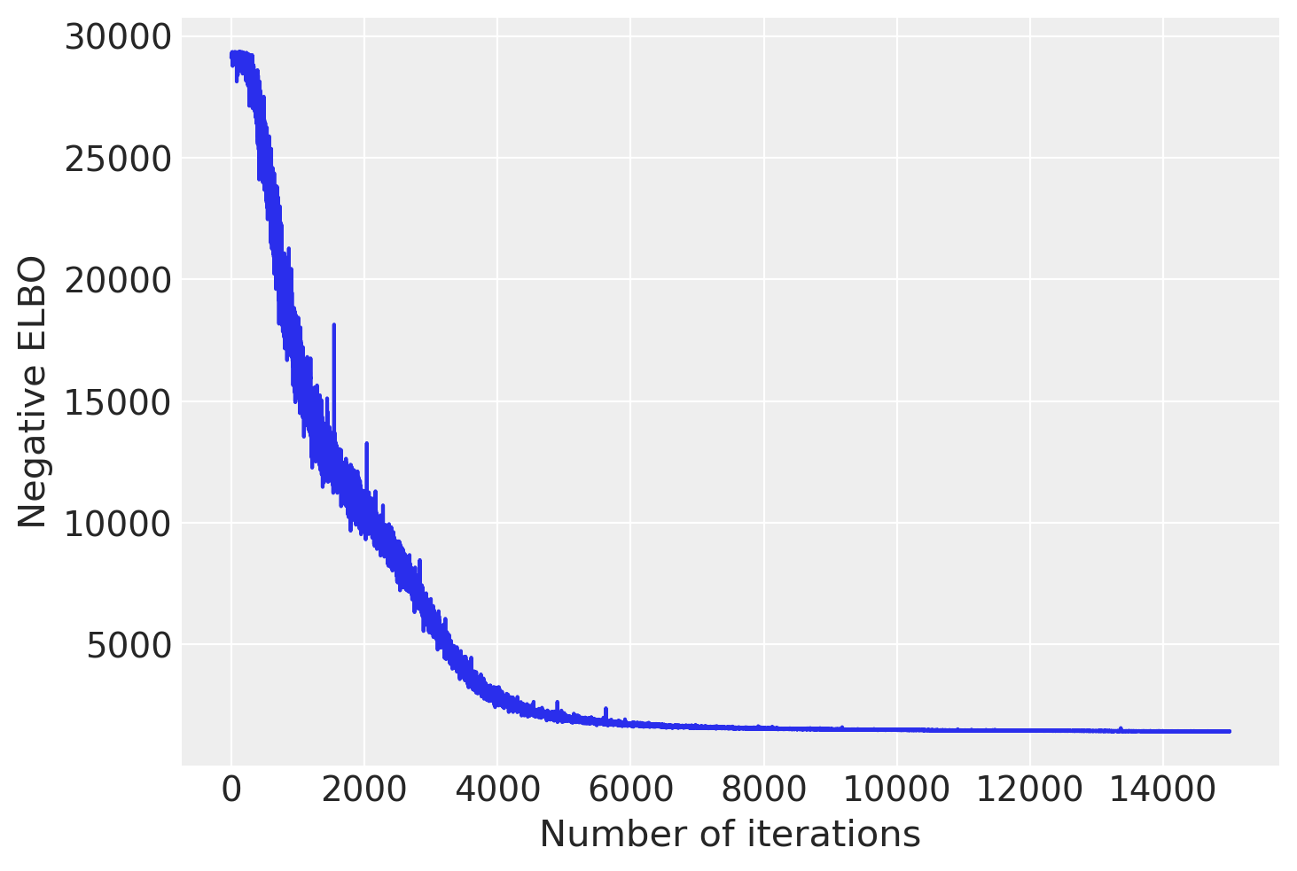
advi = pm.fit(
model,
num_steps=15000
)
plt.plot(advi.losses)
plt.xlabel('Number of iterations')
plt.ylabel('Negative ELBO')
plt.show()
trace = advi[0].sample(15000)
xx = np.asarray(trace.posterior['GPLVM/x'])
xx = xx.squeeze()
plt.scatter(xx.mean(0)[:, 0], xx.mean(0)[:, 1], c=iris.target)
plt.show()
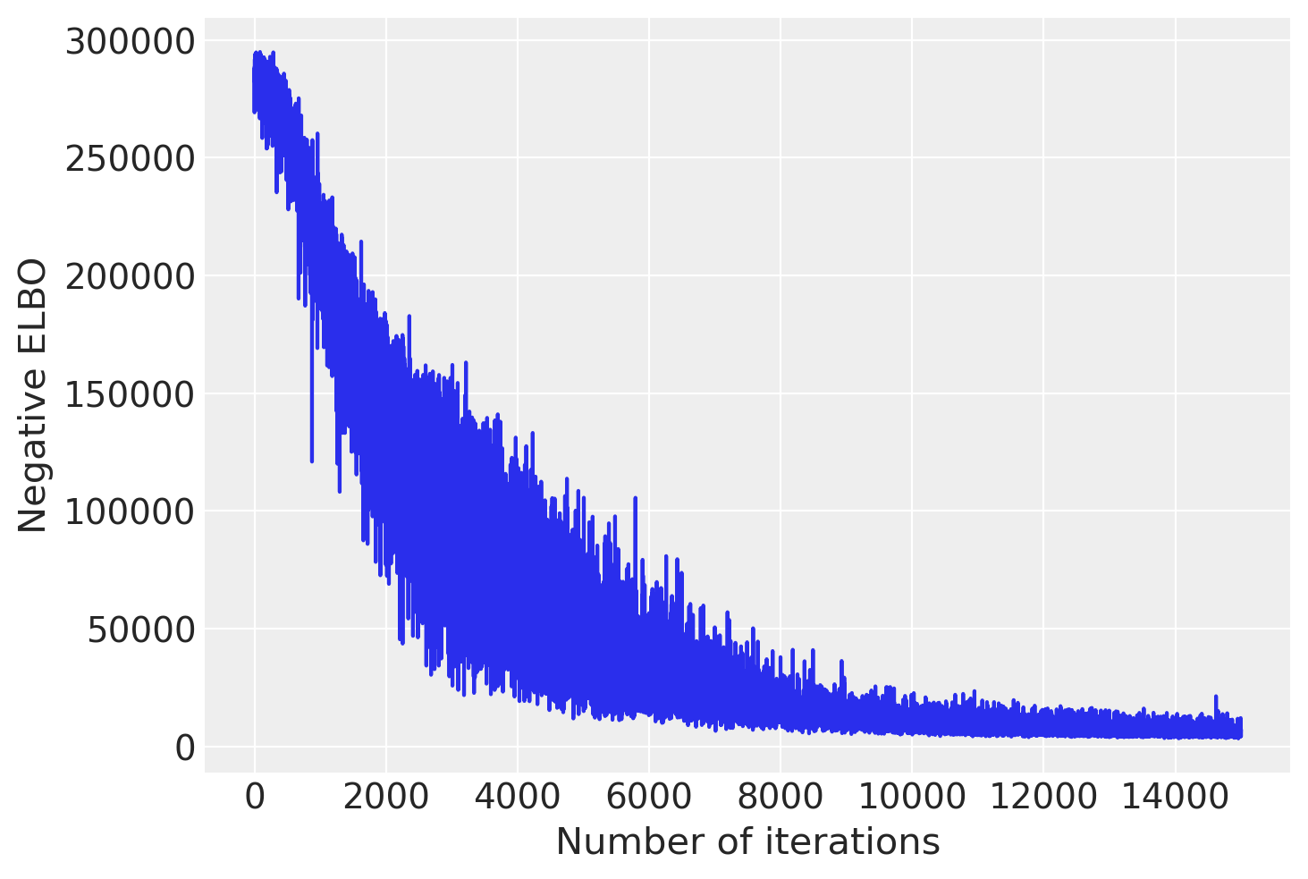
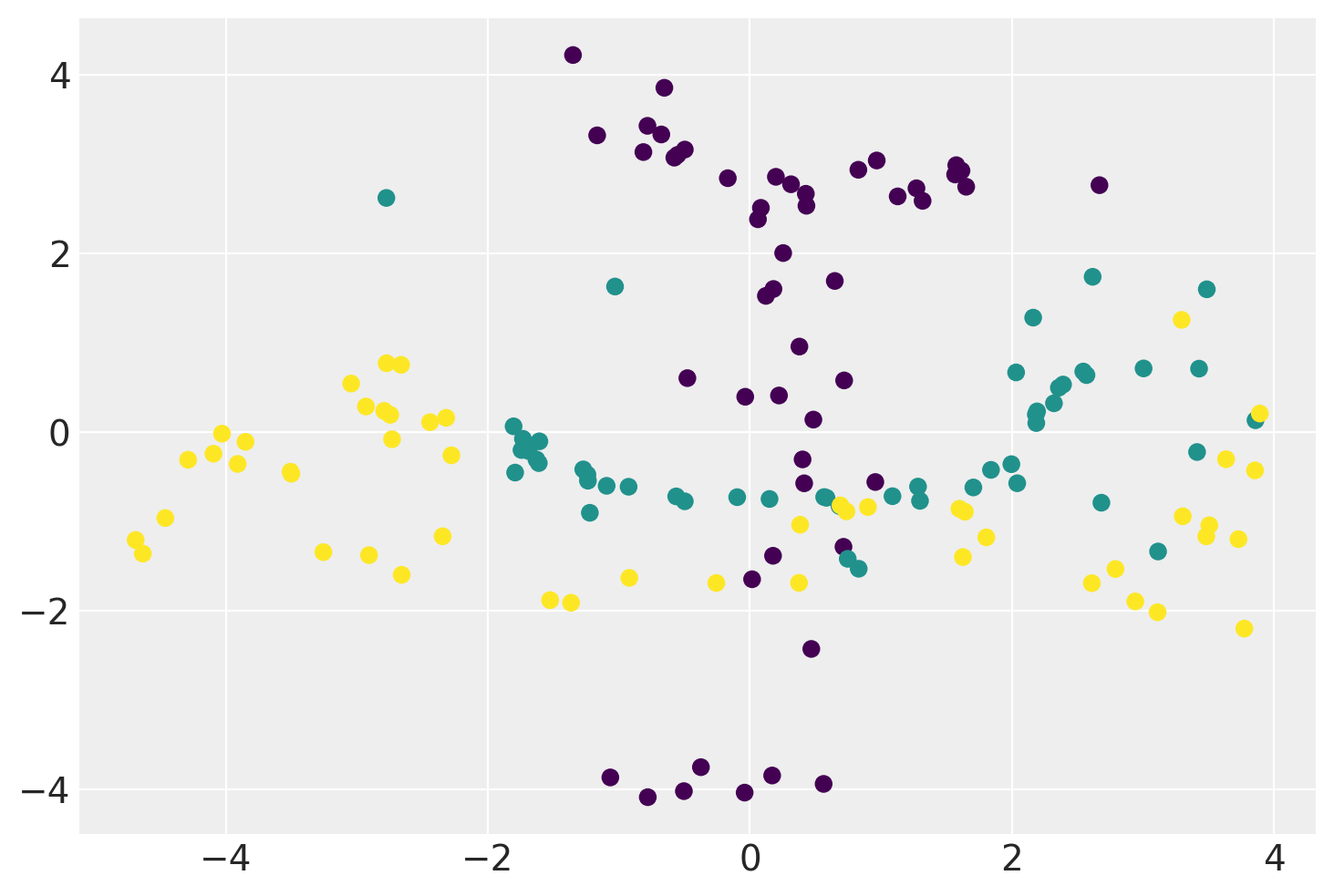
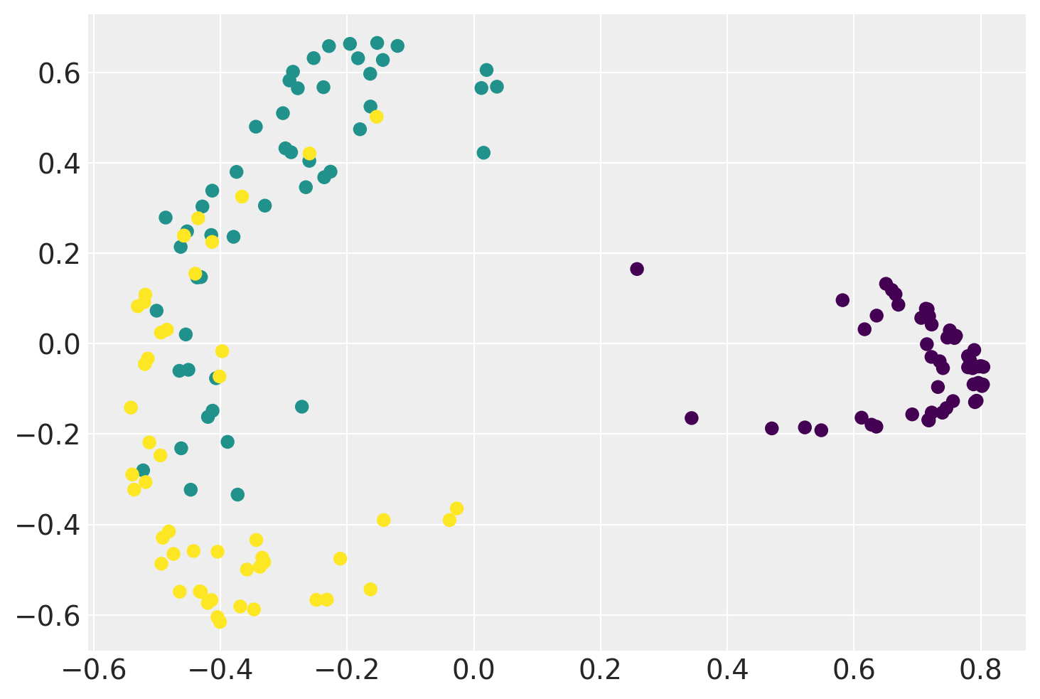
GP-LVMs with a non-linear kernel
Below is the demonstration of a GP-LVM using a non-linear RBF kernel and a comparison with the sklearn’s KernelPCA model.
# Experiments with Non-Linear Kernels
@pm.model
def GPLVM():
    # A normal prior over the projected data
    x = yield pm.MvNormalCholesky('x', loc=np.zeros(2), scale_tril=np.eye(2), batch_stack=N)

    # Prior over the argumemnts of the covariance function.
    args = yield pm.Uniform('args', np.array(1.), np.array(100.0), batch_stack=2)
    cov_fn = pm.gp.cov.ExpQuad(args[0], args[1])
    gp = pm.gp.MarginalGP(cov_fn=cov_fn)

    # We put a marginal likelihood over every feature in the dataset.
    for i in range(P):
        y = yield gp.marginal_likelihood(f'y_{i}', X=x, y=Y[:, i], noise=np.array(1e-3))

model = GPLVM()
advi = pm.fit(model, num_steps=15000)

plt.plot(advi.losses)
plt.xlabel('Number of iterations')
plt.ylabel('Negative ELBO')
plt.show()

trace = advi[0].sample(15000)

xx = np.asarray(trace.posterior['GPLVM/x'])
xx = xx.squeeze()

plt.scatter(xx.mean(0)[:, 0], xx.mean(0)[:, 1], c=iris.target)
plt.show()
# Comparing with sklearn
transformer = KernelPCA(n_components=2, kernel='rbf')
xx = transformer.fit_transform(Y)

plt.scatter(xx[:, 0], xx[:, 1], c=iris.target)
plt.show()
%load_ext watermark
%watermark -n -u -v -iv -w
pymc4      4.0a2
arviz      0.9.0
tensorflow 2.4.0-dev20200705
numpy      1.19.0
last updated: Fri Aug 07 2020

CPython 3.8.0
IPython 7.16.1
watermark 2.0.2